1.数据来源：

J. Nathan Kutz  Steven L. Brunton  Data-Driven Modeling of Complex Systems

网站链接：http://dmdbook.com/

CYLINDER_ALL.mat - 包含 151 个速度（u 和 v）以及涡度（UALL、VALL、VORTALL）的快照。另包含一个用于测试的额外快照。（快照分辨率 449 x 199）

注：.mat为MATLAB软件专用的数据存储标准格式

       PyVista: 一个的 Python 库，它是 VTK 的封装。这两年的视频和专栏里面有提到。用来保存重构后的结果。VTK作为开源库，其格式更能被各大后处理软件接受。

数据来源

2.Python代码实现

代码块

Python

     自动换行
   

     复制代码
   

123456789101112131415161718192021222324252627282930313233343536373839404142434445464748495051525354555657585960616263646566676869707172737475767778798081828384858687888990919293949596979899100101102103104105106107108109110111112113114115116117118119120121122123124125126127128129130131132133134135136137138139140141142143144145146147148149150151152153154155156157158159160161162163164165166167168169170171172173174175176177178179180181182183184185186187188189190191192193194195196197198199200201202203204205206207208209210211212213214215216217218219220221222223224225226227228229230231232233234235236237238239240241242243244245246247248249250251252253254255256257258259260261262263264265266267268

# -*- coding: utf-8 -*-
"""
圆柱绕流真实数据 POD 分析 

数据: CYLINDER_ALL.mat (449x199, 151 snapshots)  
      from J. Nathan Kutz & Steven L. Brunton
依赖: EX16.py (PODROM类)

- 自动检测数据格式 (2D/3D)
- 兼容不同的MATLAB导出格式

@author: bzhan666
"""

import numpy as np
import pyvista as pv
from pathlib import Path
import matplotlib.pyplot as plt
from scipy.io import loadmat
from EX16 import PODROM

plt.rcParams['font.sans-serif'] = ['SimHei', 'DejaVu Sans']
plt.rcParams['axes.unicode_minus'] = False


class RealDataBridge:
    """读取 MATLAB数据 """
    
    def __init__(self, output_dir="./cylinder_vtk"):
        self.output_dir = Path(output_dir)
        self.output_dir.mkdir(exist_ok=True)
        self.mesh = None
        self.grid_shape = None

    def load_cylinder_mat_data(self, mat_file="CYLINDER_ALL.mat", variable='VORTALL'):
        """
        加载圆柱绕流 .mat 数据 (自动检测格式)
        
        Args:
            mat_file: 文件路径
            variable: 'VORTALL', 'UALL', 'VALL'
        
        Returns:
            snapshots: (n_space, n_time)
            grid_shape: (nx, ny)
        """
        print("="*70)
        print(f"加载 {mat_file}")
        print("="*70)
        
        # 读取文件
        mat_data = loadmat(mat_file)
        
        # 显示文件内容
        print("\n文件内容:")
        for key in mat_data.keys():
            if not key.startswith('__'):
                print(f"  {key}: {mat_data[key].shape}")
        
        field_data = mat_data[variable]
        print(f"\n目标变量: {variable}")
        print(f"原始形状: {field_data.shape}")
        
        # 自动检测数据格式
        if field_data.ndim == 3:
            # 格式1: (ny, nx, nt) 或 (nx, ny, nt)
            dim1, dim2, nt = field_data.shape
            print(f"检测到3D数组: ({dim1}, {dim2}, {nt})")
            
            # 判断哪个是 nx (通常 nx > ny)
            if dim2 > dim1:
                ny, nx = dim1, dim2
                print(f"推断: ny={ny}, nx={nx}, nt={nt}")
            else:
                nx, ny = dim1, dim2
                print(f"推断: nx={nx}, ny={ny}, nt={nt}")
            
            # 转为快照矩阵 (n_space, nt)
            snapshots = field_data.reshape(-1, nt, order='F')
            self.grid_shape = (nx, ny)
            
        elif field_data.ndim == 2:
            # 格式2: (n_space, nt) 已经是快照矩阵
            n_space, nt = field_data.shape
            print(f"检测到2D数组: ({n_space}, {nt})")
            snapshots = field_data
            
            # 推断网格尺寸 (根据描述应该是 449x199)
            # 尝试因式分解
            nx = 449  # 从描述得知
            ny = n_space // nx
            
            if nx * ny != n_space:
                # 如果不匹配,尝试接近正方形
                nx = int(np.sqrt(n_space * 2.25))  # 假设 nx:ny ≈ 2.25:1
                ny = n_space // nx
            
            print(f"推断网格: {nx} x {ny}")
            self.grid_shape = (nx, ny)
            
        else:
            raise ValueError(f"不支持的数据维度: {field_data.ndim}")
        
        print(f"\n最终:")
        print(f"  网格: {nx} x {ny} = {nx*ny:,} 点")
        print(f"  时间步: {nt}")
        print(f"  快照矩阵: {snapshots.shape}")
        print(f"  数值范围: [{snapshots.min():.2f}, {snapshots.max():.2f}]")
        
        # 创建 VTK 网格
        x = np.linspace(0, 10, nx)
        y = np.linspace(-2, 2, ny)
        xx, yy = np.meshgrid(x, y, indexing='xy')
        zz = np.zeros_like(xx)
        self.mesh = pv.StructuredGrid(xx, yy, zz)
        
        print("\n数据加载完成\n")
        return snapshots, (nx, ny)

    def save_to_vtk(self, field_vector, filename, field_name="Field"):
        """保存场到 VTK"""
        grid = self.mesh.copy()
        grid.point_data[field_name] = field_vector
        grid.save(self.output_dir / filename)


def visualize_modes(rom, grid_shape, n_show=6, save_path=None):
    """可视化 POD 模态"""
    nx, ny = grid_shape
    fig, axes = plt.subplots(2, 3, figsize=(15, 10))
    axes = axes.ravel()
    
    for i in range(n_show):
        mode = rom.modes[:, i].reshape(ny, nx)
        vmax = np.abs(mode).max()
        
        im = axes[i].imshow(mode, cmap='RdBu_r', aspect='auto', vmin=-vmax, vmax=vmax)
        axes[i].set_title(f'Mode {i+1} (σ={rom.singular_values[i]:.2f})', fontsize=12, fontweight='bold') axes[i].axis('off') plt.colorbar(im, ax=axes[i], fraction=0.046) plt.tight_layout() if save_path: plt.savefig(save_path, dpi=200, bbox_inches='tight') print(f" 模态图已保存: {save_path}") plt.show() def visualize_energy(rom, save_path=None): """可视化能量谱""" s = rom.singular_values energy = s**2 cumulative = np.cumsum(energy) / np.sum(energy) * 100 fig, (ax1, ax2) = plt.subplots(1, 2, figsize=(14, 5)) # 奇异值衰减 ax1.semilogy(range(1, len(s)+1), s, 'bo-', markersize=6) ax1.set_xlabel('模态数', fontsize=12) ax1.set_ylabel('奇异值', fontsize=12) ax1.set_title('奇异值衰减', fontsize=13, fontweight='bold') ax1.grid(True, alpha=0.3) # 累积能量 ax2.plot(range(1, len(s)+1), cumulative, 'r^-', markersize=6) ax2.axhline(90, color='gray', linestyle='--', alpha=0.5, label='90%') ax2.axhline(99, color='green', linestyle='--', alpha=0.5, label='99%') ax2.set_xlabel('模态数', fontsize=12) ax2.set_ylabel('累积能量 (%)', fontsize=12) ax2.set_title('能量收敛', fontsize=13, fontweight='bold') ax2.legend() ax2.grid(True, alpha=0.3) plt.tight_layout() if save_path: plt.savefig(save_path, dpi=200, bbox_inches='tight') print(f"能量图已保存: {save_path}") plt.show() def main(): """主函数""" print("="*70) print(" 圆柱绕流 POD 分析 (单场)") print("="*70) print() # === 配置 === MAT_FILE = "CYLINDER_ALL.mat" VARIABLE = 'VORTALL' # 可选: 'UALL', 'VALL', 'VORTALL' N_MODES = 20 N_TRAIN = 150 # 用前150个训练 N_EXPORT = 30 # 导出30个快照 # === 步骤1: 加载数据 === bridge = RealDataBridge() snapshots, grid_shape = bridge.load_cylinder_mat_data(MAT_FILE, VARIABLE) # 分割训练/测试 train_data = snapshots[:, :N_TRAIN] test_data = snapshots[:, N_TRAIN:] # === 步骤2: 训练 POD === print("="*70) print("训练 POD 模型") print("="*70) rom = PODROM(n_modes=N_MODES) rom.fit(train_data) # === 步骤3: 评估 === print("\n" + "="*70) print("性能评估") print("="*70) # 训练集误差 train_error = rom.compute_reconstruction_error(train_data, 'relative') print(f"训练集相对误差: {train_error:.6f} ({train_error*100:.4f}%)") # 测试集误差 if test_data.shape[1] > 0: test_error = rom.compute_reconstruction_error(test_data, 'relative') print(f"测试集相对误差: {test_error:.6f} ({test_error*100:.4f}%)") # === 步骤4: 可视化 === print("\n" + "="*70) print("生成可视化") print("="*70) visualize_modes(rom, grid_shape, n_show=6, save_path=bridge.output_dir/'modes.png') visualize_energy(rom, save_path=bridge.output_dir/'energy.png') # === 步骤5: 导出 VTK === print("\n" + "="*70) print("导出 VTK 文件") print("="*70) n_export = min(N_EXPORT, N_TRAIN) print(f"导出前 {n_export} 个时间步...\n") for i in range(n_export): original = train_data[:, i] reconstructed = rom.reconstruct(original) error = original - reconstructed bridge.save_to_vtk(original, f"orig_{i:04d}.vtk", f"{VARIABLE}_Original") bridge.save_to_vtk(reconstructed, f"recon_{i:04d}.vtk", f"{VARIABLE}_Recon") bridge.save_to_vtk(error, f"error_{i:04d}.vtk", f"{VARIABLE}_Error") if (i + 1) % 10 == 0: print(f" 进度: {i+1}/{n_export}") print(f"\n VTK 文件已保存到: {bridge.output_dir.absolute()}") # === 结论 === print("\n" + "="*70) print("分析完成") print("="*70) print(f"输出目录: {bridge.output_dir}") return rom, bridge if __name__ == "__main__": rom, bridge = main()
        
      复制成功
     
     
     
     

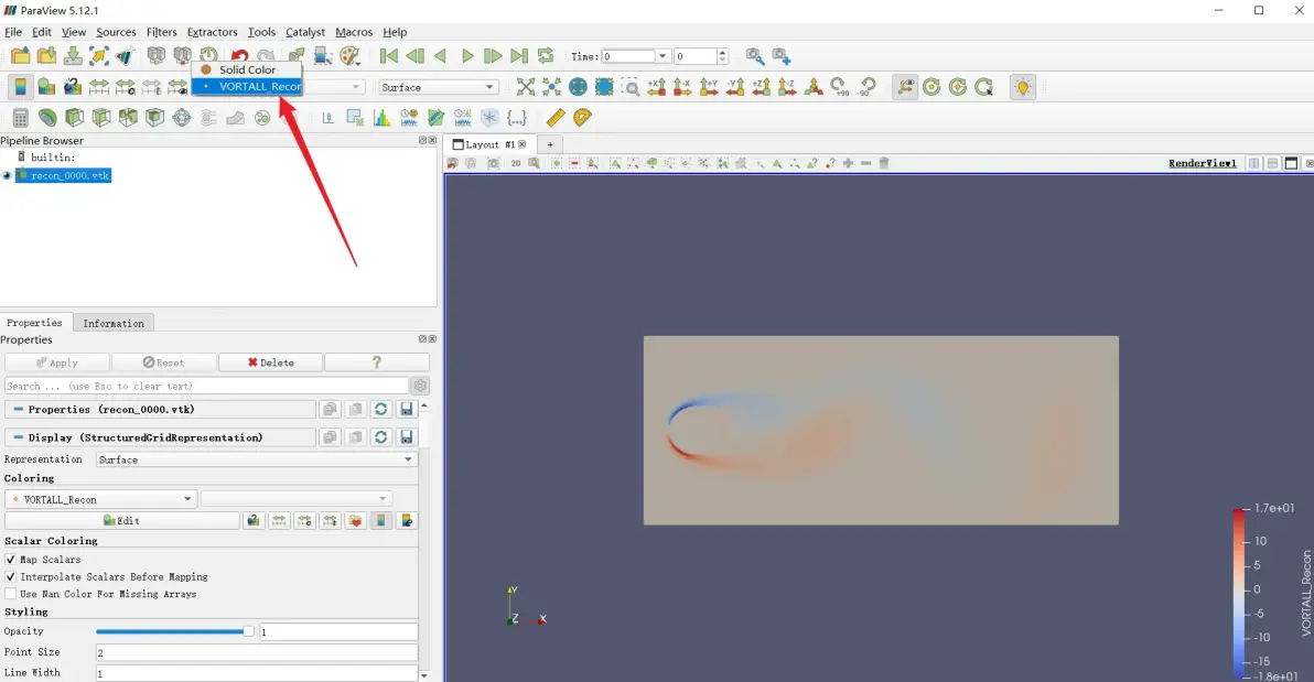
Paraview中看单一变量

重构后云图

重构后与云图误差

免责声明：本文系网络转载或改编，未找到原创作者，版权归原作者所有。如涉及版权，请联系删