matlab实验无限冲激响应IIR数字滤波器设计

一、实验目的

1、掌握构成一个频率响应与给定的滤波特性相接近的模拟滤波器的设计原理。

2、掌握用冲激响应不变法设计IIR数字滤波器的基本原理。

3、了解数字滤波器和模拟滤波器的频率响应特性，掌握相应的计算方法，分析用冲激响应不变法获得的数字滤波器频率响应特性中出现的混叠现象。

4、掌握用双线性变换法设计IIR数字滤波器的基本原理和算法。

二、实验原理

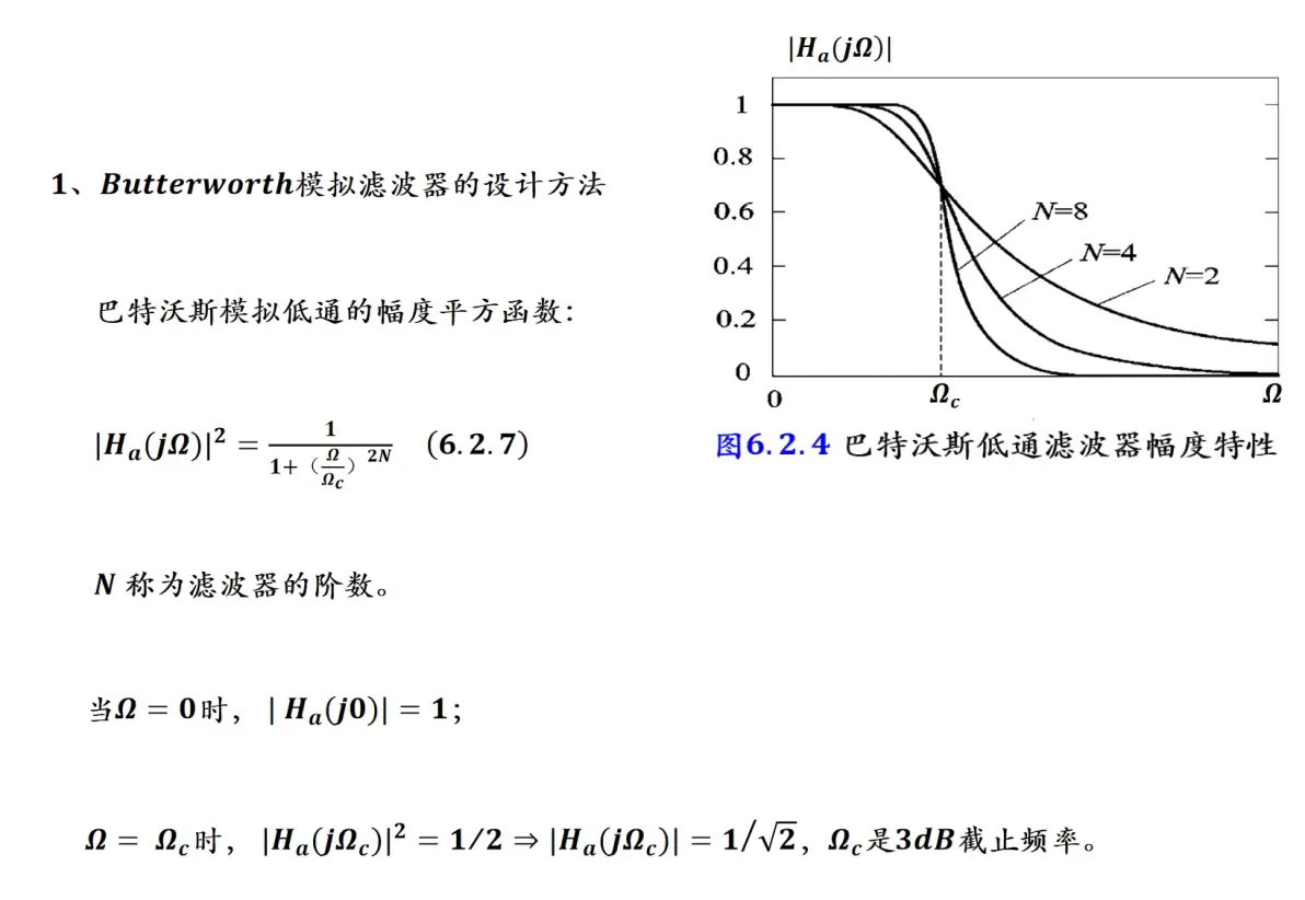
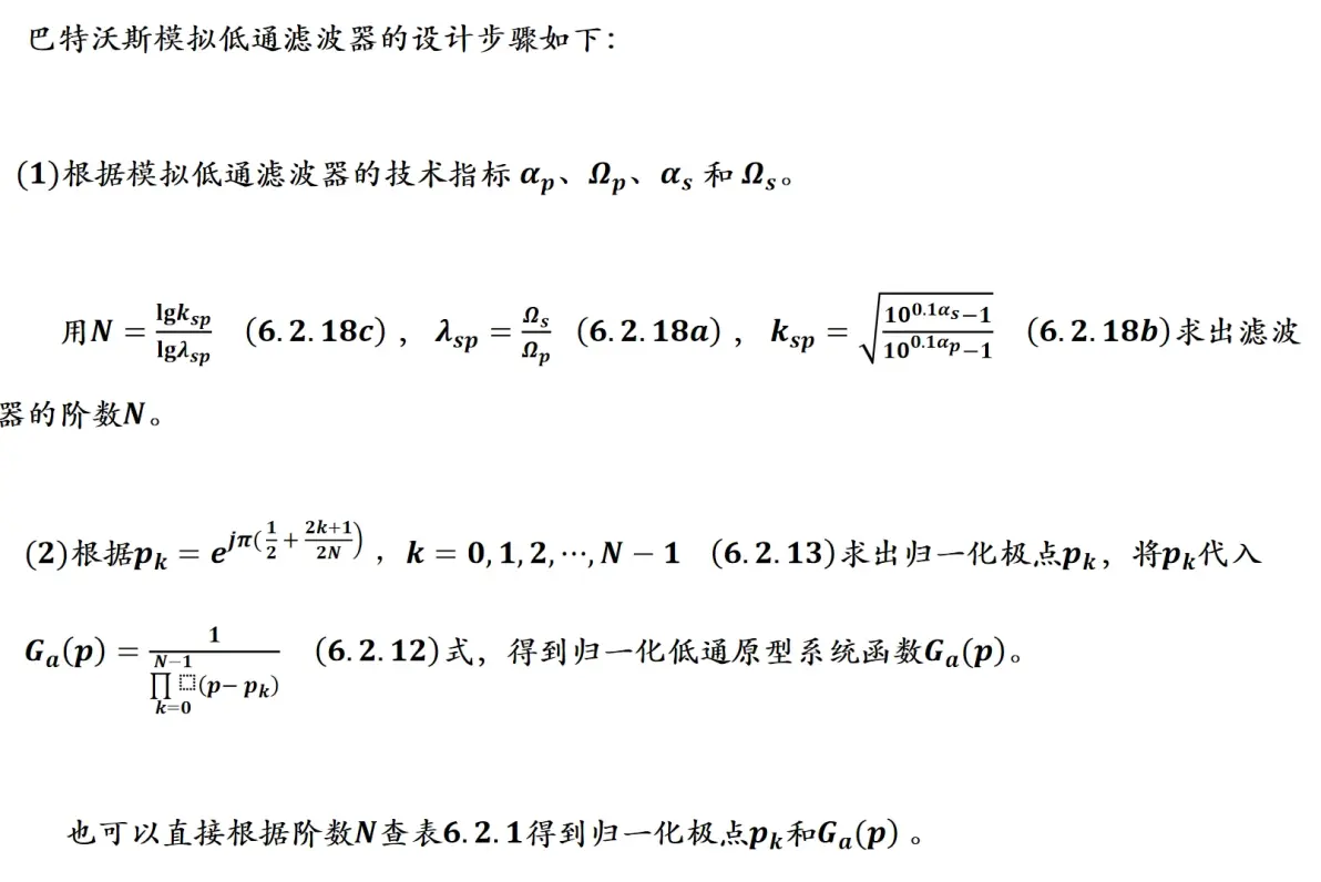
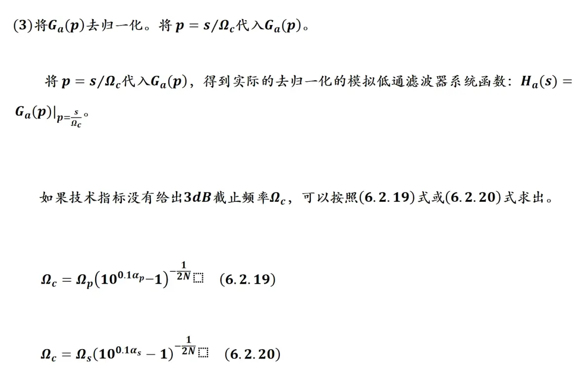
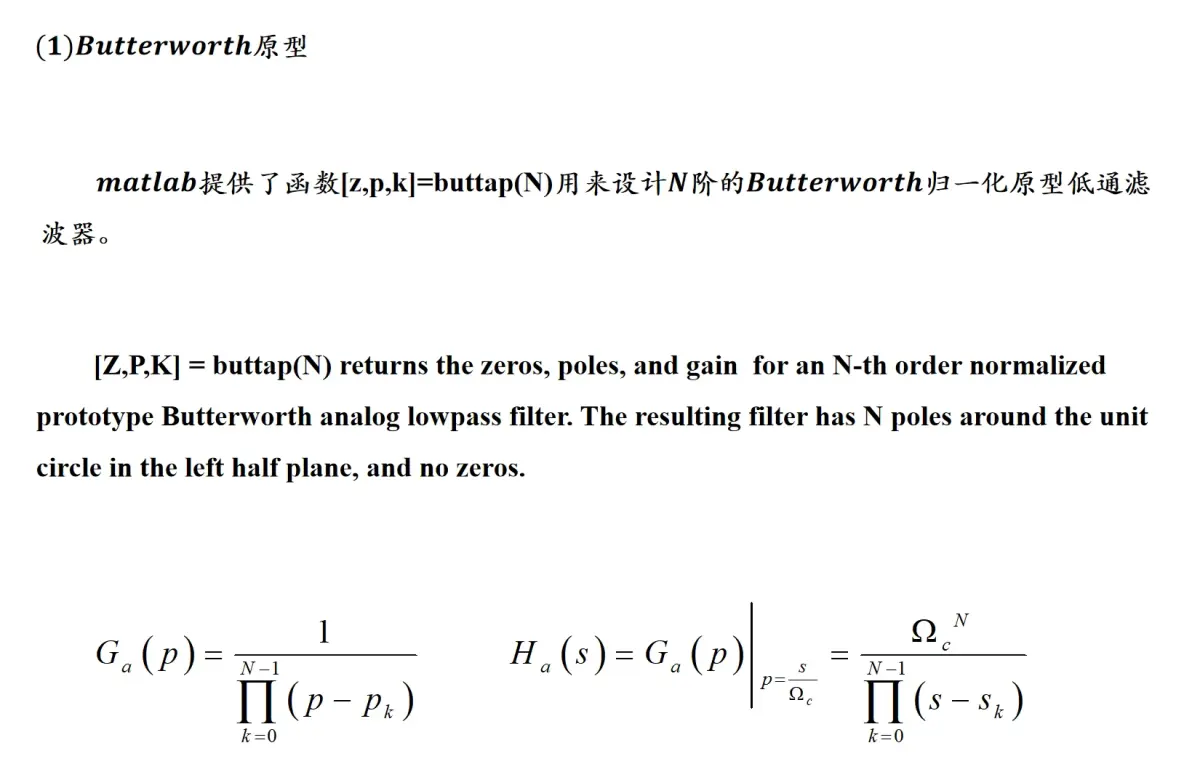
自编函数[b,a]=u_buttap(N,Omegac)给出未归一化的Butterworth模拟低通滤波器。

function [b,a] = u_buttap(N,Omegac);

% Unnormalized Butterworth Analog Lowpass Filter Prototype

% [b,a] = u_buttap(N,Omegac);

% b = numerator polynomial coefficients of Ha(s)

% a = denominator polynomial coefficients of Ha(s)

% N = Order of the Butterworth Filter

% Omegac = Cutoff frequency in radians/sec

[z,p,k] = buttap(N);

p = p*Omegac;

k = k*Omegac^N;

B = real(poly(z));

b0 = k;

b = k*B;

a = real(poly(p));

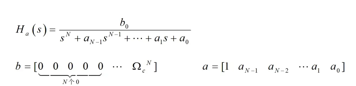
   poly(V), when V is a vector, is a vector whose elements are the coefficients of the polynomial whose roots are the elements of V. For vectors, ROOTS and poly are inverse functions of each other, up to ordering, scaling, and roundoff error.

可以利用函数[C,B,A]=sdir2cas(b,a)得到级联形式的N阶Butterworth模拟低通滤波器。

模拟滤波器直接型转级联形式

function [C,B,A] = sdir2cas(b,a);

% DIRECT-form to CASCADE-form conversion in s-plane

% [C,B,A] = sdir2cas(b,a)

% C = gain coefficient

% B = K by 3 matrix of real coefficients containing bk's

% A = K by 3 matrix of real coefficients containing ak's

% b = numerator polynomial coefficients of DIRECT form

% a = denominator polynomial coefficients of DIRECT form

Na = length(a)-1; Nb = length(b)-1;

% compute gain coefficient C

b0 = b(1); b = b/b0;

a0 = a(1); a = a/a0;

C = b0/a0;

% Denominator second-order sectio

if K*2 == Na % Computation when Na is even

A = zeros(K,3);

for n=1:2:Na

Arow = p(n:1:n+1,:);

Arow = poly(Arow);

A(fix((n+1)/2),:) = real(Arow);

end

elseif Na == 1 % Computation when Na = 1

A = [0 real(poly(p))];

else % Computation when Na is odd and > 1

A = zeros(K+1,3);

for n=1:2:2*K

Arow = p(n:1:n+1,:);

Arow = poly(Arow);

A(fix((n+1)/2),:) = real(Arow);

end

A(K+1,:) = [0 real(poly(p(Na)))];

end

% Numerator second-order sections:

z = cplxpair(roots(b)); K = floor(Nb/2);

if Nb == 0 % Computation when Nb = 0

B = [0 0 poly(z)];

elseif K*2 == Nb % Computation when Nb is even

B = zeros(K,3);

for n=1:2:Nb

Brow = z(n:1:n+1,:);

Brow = poly(Brow);

B(fix((n+1)/2),:) = real(Brow);

end

elseif Nb == 1 % Computation when Nb = 1

B = [0 real(poly(z))];

else % Computation when Nb is odd and > 1

B = zeros(K+1,3);

for n=1:2:2*K

Brow = z(n:1:n+1,:);

Brow = poly(Brow);

B(fix((n+1)/2),:) = real(Brow);

end

B(K+1,:) = [0 real(poly(z(Nb)))];

end

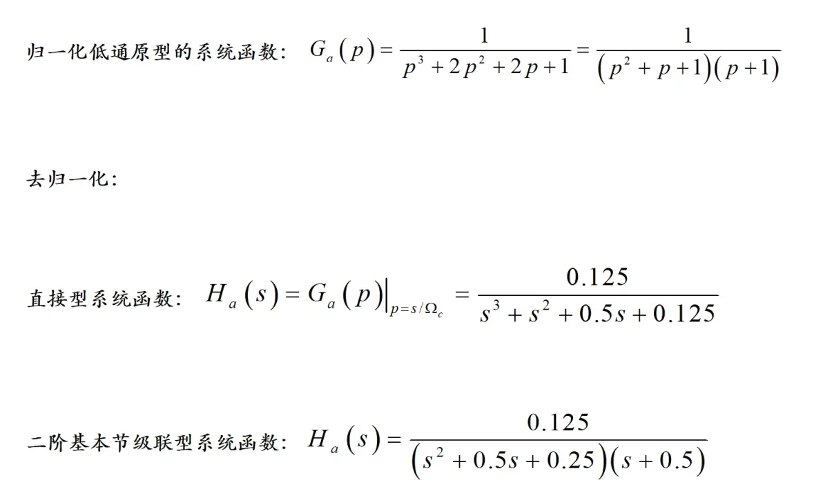
例1：3阶Butterworth原型模拟低通的3dB截止频率Ω_c=0.5，求非归一化的系统函数H_a(s)。

%程序eg_2.m

N=3;

OmegaC=0.5;

[b,a]=u_buttap(N,OmegaC) %去归一化巴特沃斯低通系统函数分子、分母多项式系数向量

[C,B,A]=sdir2cas(b,a) %直接型转换为级联型

直接型系数：

b =

 0.1250

a =

 1.0000  1.0000  0.5000  0.1250

级联型系数：

C =

 0.1250

B =

  0   0   1

A =

 1.0000  0.5000  0.2500

    0    1.0000   0.5000

(2)按给定技术指标设计Butterworth模拟低通滤波器

已知模拟低通的技术指标： α_p、Ω_p、α_s 和 Ω_s。

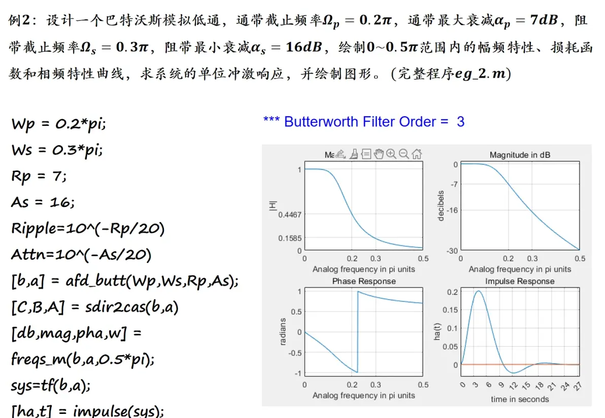
(a)函数[b,a]=afd_butt(Wp,Ws,Rp,As)：按给定技术指标设计Butterworth模拟低通滤波器；

(b)函数[db,mag,pha,w]=freqs_m(b,a, wmax)：求模拟滤波器得出衰减值、幅频特性、相频特性和频率向量w；

(c)[ha,t]=impulse(sys)： 求模拟滤波器的单位冲激响应，可以用plot(t,ha)命令画出单位冲激响应曲线。

(a)函数[b,a]=afd_butt(Wp,Ws,Rp,As)

function [b,a] = afd_butt(Wp,Ws,Rp,As);

% Analog Lowpass Filter Design: Butterworth

% [b,a] = afd_butt(Wp,Ws,Rp,As);

% b = Numerator coefficients of Ha(s)

% a = Denominator coefficients of Ha(s)

% Wp = Passband edge frequency in rad/sec; Wp > 0

% Ws = Stopband edge frequency in rad/sec; Ws > Wp > 0

% Rp = Passband ripple in +dB; (Rp > 0)

% As = Stopband attenuation in +dB; (As > 0)

if Ws <= Wp

error('Stopband edge must be larger than Passband edge')

end

if (Rp <= 0) | (As < 0)

error('PB ripple and/or SB attenuation ust be larger than 0')

end

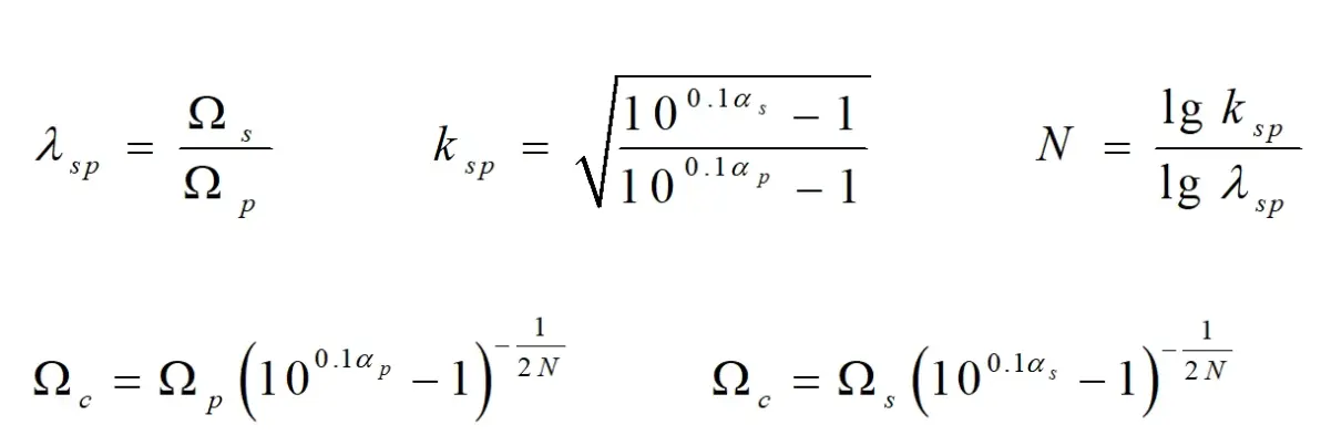
N = ceil((log10((10^(Rp/10)-1)/(10^(As/10)-1)))/(2*log10(Wp/Ws)));

fprintf('\n*** Butterworth Filter Order = %2.0f \n',N)

OmegaC = Wp/((10^(Rp/10)-1)^(1/(2*N)));

[b,a]=u_buttap(N,OmegaC);

(1)ceil、round、floor、fix的区别：

(a) ceil(x)：向正方向取整

(b) round(x)：四舍五入

(c) floor(x)：向负方向取整

(d) fix(x)：取整数部分

>> x=[-1.6  -1.4  1.4  1.6  3];

>> ceil(x)

ans =

 -1  -1   2   2   3

>> round(x)

ans =

 -2  -1   1   2   3

>> floor(x)

ans =

 -2  -2   1   1   3

>> fix(x)

ans =

 -1  -1   1   1   3

(b)函数[db,mag,pha,w]=freqs_m(b,a, wmax)

function [db,mag,pha,w] = freqs_m(b,a,wmax);

% Computation of s-domain frequency response: Modified version

% [db,mag,pha,w] = freqs_m(b,a,wmax);

% db = Relative magnitude in db over [0 to wmax]

% mag = Absolute magnitude over [0 to wmax]

% pha = Phase response in radians over [0 to wmax]

% w = array of 500 frequency samples between [0 to wmax]

% b = Numerator polynomial coefficents of Ha(s)

% a = Denominator polynomial coefficents of Ha(s)

% wmax = Maximum frequency in rad/sec over which response is desired

w = [0:1:500]*wmax/500;

H = freqs(b,a,w);

mag = abs(H);

db = 20*log10((mag+eps)/max(mag));

pha = angle(H);

H = freqs(B,A,W) returns the complex frequency response vector H of the filter B/A:

               nb-1     nb-2

      B(s)  b(1)s   + b(2)s   + ... + b(nb)

  H(s) = ---- = -------------------------------------

               na-1     na-2

      A(s)  a(1)s   + a(2)s   + ... + a(na)

 given the numerator and denominator coefficients in vectors B and A.The frequency response is evaluated at the points specified in vector W (in rad/s). The magnitude and phase can be graphed by calling freqs(B,A,W) with no output arguments.

(c)[ha,t]=impulse(sys)

[Y,T] = impulse(SYS)

 returns the output response Y and the time vector T used for simulation.No plot is drawn on the screen. If SYS has NY outputs and NU inputs, and LT=length(T), Y is an array of size [LT NY NU] where Y(:,:,j) gives the impulse response of the j-th input channel. The time vector T is

expressed in the time units of SYS.

sys=tf(b,a);

2、Chebyshev I型模拟滤波器的设计方法

(1)Chebyshev I型原型

函数[z,p,k]=cheb1ap(N,Rp)：用来设计N阶通带波纹幅度为Rp的Chebyshev I型归一化模拟低通滤波器；

函数[b,a]=u_chb1ap(N,Rp,OmegaP)给出未归一化的Chebyshev I型模拟低通滤波器。

function [b,a] = u_chb1ap(N,Rp,OmegaP);

% Unnormalized Chebyshev-1 Analog Lowpass Filter Prototype

% [b,a] = u_chb1ap(N,Rp,OmegaP);

% b = numerator polynomial coefficients

% a = denominator polynomial coefficients

% N = Order of the Elliptic Filter

% Rp = Passband Ripple in dB; Rp > 0

% OmegaP = Cutoff frequency in radians/sec

[z,p,k] = cheb1ap(N,Rp);

a = real(poly(p));aNn = a(N+1);

p = p*OmegaP;

a = real(poly(p));aNu = a(N+1);

k = k*aNu/aNn;b0 = k;

B = real(poly(z));

b = k*B;

2、Chebyshev I型模拟滤波器的设计方法

(2)按给定技术指标设计Chebyshev I型模拟低通滤波器

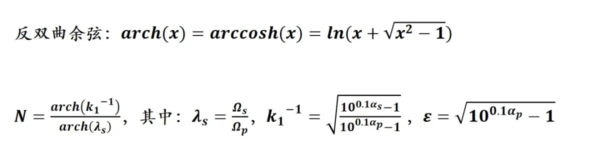
   函数[b,a]=afd_chb1(Wp,Ws,Rp,As)：用来实现按给定技术指标设计Chebyshev I型模拟低通滤波器。

function [b,a] = afd_chb1(Wp,Ws,Rp,As);

% Analog Lowpass Filter Design: Chebyshev-1

% [b,a] = afd_chb1(Wp,Ws,Rp,As);

% b = Numerator coefficients of Ha(s)

% a = Denominator coefficients of Ha(s)

% Wp = Passband edge frequency in rad/sec; Wp > 0

% Ws = Stopband edge frequency in rad/sec; Ws > Wp > 0

% Rp = Passband ripple in +dB; (Rp > 0)

% As = Stopband attenuation in +dB; (

if Wp <= 0

error('Passband edge must be larger than 0')

end

if Ws <= Wp

error('Stopband edge must be larger than Passband edge')

end

if (Rp <= 0) | (As < 0)

error('PB ripple and/or SB attenuation ust be larger than 0')

end

ep = sqrt(10^(Rp/10)-1);

A = 10^(As/20);

OmegaC = Wp;

OmegaR = Ws/Wp;

g = sqrt(A*A-1)/ep;

N = ceil(log10(g+sqrt(g*g-1))/log10(OmegaR+sqrt(OmegaR*OmegaR-1)));

fprintf('\n*** Chebyshev-1 Filter Order = %2.0f \n',N)

[b,a]=u_chb1ap(N,Rp,OmegaC);

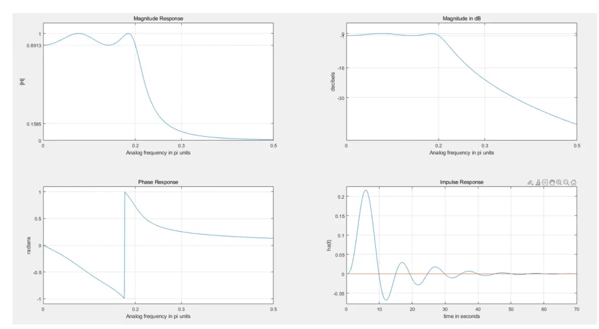
例3：设计一个切比雪夫I型模拟低通，通带截止频率Ω_p=0.2π，通带最大衰减α_p=1dB，阻带截止频率Ω_s=0.3π，阻带最小衰减α_s=16dB，绘制0~0.5π范围内的幅频特性曲线、损耗函数曲线和相频特性曲线，求系统的冲激响应，并绘制图形。

Wp = 0.2*pi;

Ws = 0.3*pi; Rp = 1; As = 16; Ripple = 10 ^ (-Rp/20); Attn = 10 ^ (-As/20); [b,a] = afd_chb1(Wp,Ws,Rp,As); [C,B,A] = sdir2cas(b,a) [db,mag,pha,w] = freqs_m(b,a,0.5*pi); sys=tf(b,a);

[ha,t] = impulse(sys);

%绘图参考程序eg_3.m

3、模拟滤波器到数字滤波器的变换

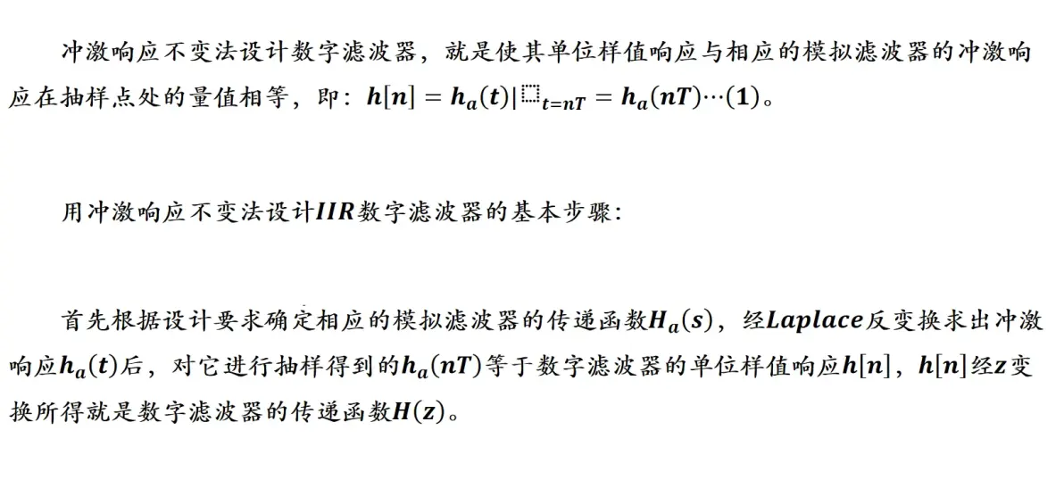
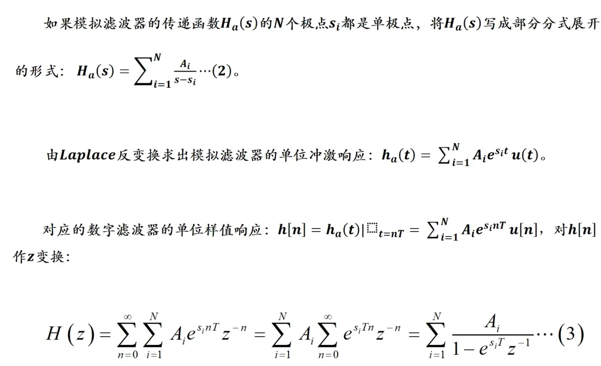
(1)冲激响应不变法设计 IIR数字滤波器的基本原理

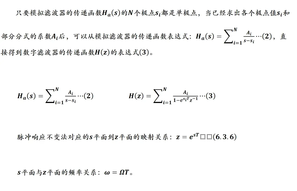
function [b,a] = imp_invr(c,d,T)

% Impulse Invariance Transformation from Analog to Digital Filter

% [b,a] = imp_invr(c,d,T)

% b = Numerator polynomial in z^(-1) of the digital filter

% a = Denominator polynomial in z^(-1) of the digital filter

% c = Numerator polynomial in s of the analog filter

% d = Denominator polynomial in s of the analog filter

% T = Sampling (transformation) parameter

[R,p,k] = residue(c,d);

p = exp(p*T);

[b,a] = residuez(R,p,k);

b = real(b);

a = real(a);

[R,P,K] = residue(B,A) finds the residues, poles and direct term of

 a partial fraction expansion of the ratio of two polynomials B(s)/A(s).

 If there are no multiple roots,

   B(s)    R(1)    R(2)       R(n)

   ---- = -------- + -------- + ... + -------- + K(s)

   A(s)   s - P(1)  s - P(2)     s - P(n)

 Vectors B and A specify the coefficients of the numerator and denominator polynomials in descending powers of s. The residues are returned in the column vector R, the pole locations in column vector P, and the direct terms in row vector K. The number of poles is n = length(A)-1 = length(R) = length(P). The direct term coefficient vector is empty if length(B) < length(A), otherwise length(K) = length(B)-length(A)+1.

[R,P,K] = residuez(B,A) finds the residues, poles and direct terms of the partial-fraction expansion of B(z)/A(z),

   B(z)    r(1)        r(n)

   ---- = ------------ +... ------------ + k(1) + k(2)z^(-1) ...

   A(z)  1-p(1)z^(-1)    1-p(n)z^(-1)

 B and A are the numerator and denominator polynomial coefficients,respectively, in ascending powers of z^(-1). R and P are column vectors containing the residues and poles, respectively. K contains the direct terms in a row vector. The number of poles is n = length(A)-1 = length(R) = length(P) The direct term coefficient vector is empty if length(B) < length(A); otherwise,   length(K) = length(B)-length(A)+1

function [db,mag,pha,grd,w] = freqz_m(b,a);

% Modified version of freqz subroutine

% [db,mag,pha,grd,w] = freqz_m(b,a);

% db = Relative magnitude in dB computed over 0 to pi radians

% mag = absolute magnitude computed over 0 to pi radians

% pha = Phase response in radians over 0 to pi radians

% grd = Group delay over 0 to pi radians

%  w = 501 frequency samples between 0 to pi radians

%  b = numerator polynomial of H(z)  (for FIR: b=h)

%  a = denominator polynomial of H(z) (for FIR: a=[1])

[H,w] = freqz(b,a,1000,'whole');

 H = (H(1:1:501))'; w = (w(1:1:501))’;

 mag = abs(H);

 db = 20*log10((mag+eps)/max(mag));

 pha = angle(H);

 grd = grpdelay(b,a,w);

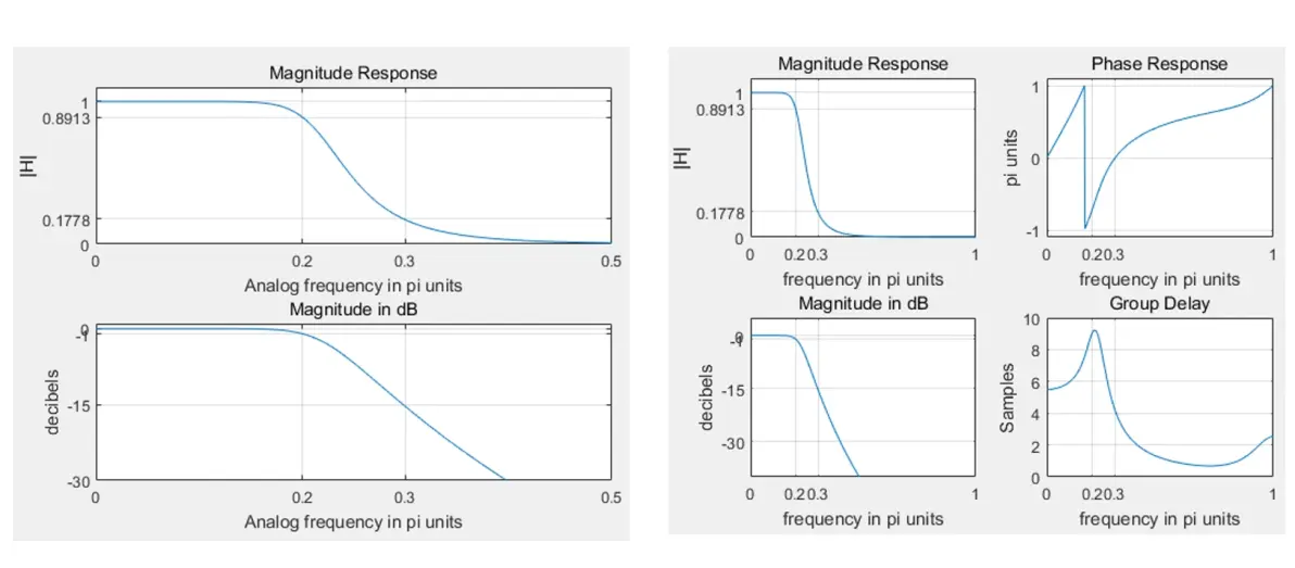
例4：利用巴特沃斯原型设计一个数字低通滤波器，通带截止频率ω_p=0.2π，通带最大衰减α_p=1dB，阻带截止频率ω_s=0.3π，阻带最小衰减α_s=15dB，绘制巴特沃斯原型低通的幅频特性和损耗函数曲线，并绘制冲激响应不变法转换得到的数字低通的幅频特性、损耗函数、相频特性曲线和群延迟。

wp = 0.2*pi; % digital Passband freq in Hz

ws = 0.3*pi; % digital Stopband freq in Hz

Rp = 1; % Passband ripple in dB

As = 15; % Stopband attenuation in dB

T = 1; % Set T=1

OmegaP = wp / T; % Prototype Passband freq

OmegaS = ws / T; % Prototype Stopband freq

ep = sqrt(10^(Rp/10)-1); % Passband Ripple parameter

Ripple = sqrt(1/(1+ep*ep)); % Passband Ripple

Attn = 1/(10^(As/20)); % Stopband

[cs,ds] = afd_butt(OmegaP,OmegaS,Rp,As);

[dbs,mags,phas,Omega] = freqs_m(cs,ds,0.5*pi);

figure(1)

subplot(211);

plot(Omega/pi,mags); grid on

title('Magnitude Response')%幅度响应线性坐标

xlabel('Analog frequency in pi units');

ylabel('|H|'); axis([0,0.5,0,1.1])

set(gca,'XTickMode','manual','XTick',[0,0.2,0.3,0.5]);%手动模式

set(gca,'YTickmode','manual','YTick',[0,Attn,Ripple,1]);

subplot(212);

plot(Omega/pi,dbs); grid on

title('Magnitude in dB')%幅度响应对数坐标

xlabel('Analog frequency in pi units');

ylabel('decibels');

axis([0,0.5,-30,1])

set(gca,'XTickMode','manual','XTick',[0,0.2,0.3,0.5]);

set(gca,'YTickmode','manual','YTick',[-30,-As,-Rp,0]);

[b,a] = imp_invr(cs,ds,T);

[C,B,A] = dir2par(b,a)

[db,mag,pha,grd,w] = freqz_m(b,a);

figure(2)

subplot(2,2,1);

plot(w/pi,mag);

grid on

title('Magnitude Response')

xlabel('frequency in pi units');

ylabel('|H|');

axis([0,1,0,1.1])

set(gca,'XTickMode','manual','XTick',[0,0.2,0.3,1]);

set(gca,'YTickmode','manual','YTick',[0,Attn,Ripple,1]);

subplot(2,2,3);

plot(w/pi,db);

title('Magnitude in dB');

xlabel('frequency in pi units');

ylabel('decibels');

axis([0,1,-40,5]);

set(gca,'XTickMode','manual','XTick',[0,0.2,0.3,1]);

set(gca,'YTickmode','manual','YTick',[-30,-As,-Rp,0]);

grid on

subplot(2,2,2);

plot(w/pi,pha/pi);

title('Phase Response')

xlabel('frequency in pi units');

ylabel('pi units');

axis([0,1,-1.1,1.1]);

set(gca,'XTickMode','manual','XTick', [0,0.2,0.3,1]);

set(gca,'YTickmode','manual','YTick',[-1,0,1]);

grid on

subplot(2,2,4);

plot(w/pi,grd);

title('Group Delay')

xlabel('frequency in pi units');

ylabel('Samples'); axis([0,1,0,10])

set(gca,'XTickMode','manual','XTick',[0,0.2,0.3,1]);

set(gca,'YTickmode','manual','YTick',[0:2:10]);

grid on

*** Butterworth Filter Order = 6

b =

 0.0000  0.0006  0.0101  0.0161  0.0041  0.0001

a =

 1.0000  -3.3635  5.0684  -4.2759  2.1066  -0.5706  0.0661

C =

  []

B =

 1.8557  -0.6304

 -2.1428  1.1454

 0.2871  -0.4466

A =

 1.0000  -0.9973  0.2570

 1.0000  -1.0691  0.3699

 1.0000  -1.2972  0.6949

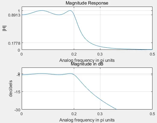
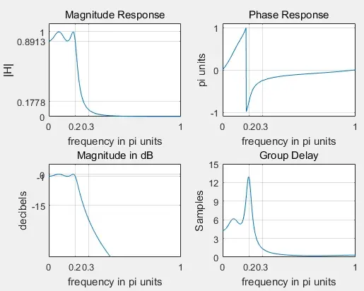
例5：利用切比雪夫I型原型低通设计数字低通，通带截止频率ω_p=0.2π，通带最大衰减α_p=1dB，阻带截止频率ω_s=0.3π，阻带最小衰减α_s=15dB，绘制切比雪夫I型原型的幅频特性和损耗函数曲线，绘制数字低通的幅频特性、损耗函数、相频特性曲线，群延迟。

wp = 0.2*pi; % digital Passband freq in Hz

ws = 0.3*pi; % digital Stopband freq in Hz

Rp = 1;   % Passband ripple in dB

As = 15;   % Stopband attenuation in dB

T = 1;    % Set T=1

OmegaP = wp / T;     % Prototype Passband freq

OmegaS = ws / T;     % Prototype Stopband freq

ep = sqrt(10^(Rp/10)-1); % Passband Ripple parameter

Ripple = sqrt(1/(1+ep*ep))% Passband Ripple

Attn = 1/(10^(As/20));  % Stopband Attenuation

[cs,ds] = afd_chb1(OmegaP,OmegaS,Rp,As);

[dbs,mags,phas,Omega] = freqs_m(cs,ds,0.5*pi);

subplot(2,1,1);

plot(Omega/pi,mags);grid on

title('Magnitude Response’)

xlabel('Analog frequency in pi units');

ylabel('|H|');

axis([0,0.5,0,1.1])

set(gca,'XTickMode','manual','XTick',[0,0.2,0.3,0.5]);

set(gca,'YTickmode','manual','YTick',[0,Attn,Ripple,1]);

subplot(2,1,2);

plot(Omega/pi,dbs);grid on

title('Magnitude in dB')

xlabel('Analog frequency in pi units');

ylabel('decibels'); axis([0,0.5,-30,5])

set(gca,'XTickMode','manual','XTick',[0,0.2,0.3,0.5]);

set(gca,'YTickmode','manual','YTick',[-30,-As,-Rp,0]);

figure;

[b,a] = imp_invr(cs,ds,T);

[C,B,A] = dir2par(b,a)

[db,mag,pha,grd,w] = freqz_m(b,a);

subplot(2,2,1);

plot(w/pi,mag);

grid on

title('Magnitude Response')

xlabel('frequency in pi units');

ylabel('|H|'); axis([0,1,0,1.1])

set(gca,'XTickMode','manual','XTick',[0,0.2,0.3,1]);

set(gca,'YTickmode','manual','YTick',[0,Attn,Ripple,1]);

subplot(2,2,3);

plot(w/pi,db);

grid on

title('Magnitude in dB');

xlabel('frequency in pi units');

ylabel('decibels'); axis([0,1,-40,5]);

set(gca,'XTickMode','manual','XTick',[0,0.2,0.3,1]);

set(gca,'YTickmode','manual','YTick',[-50,-As,-Rp,0]);

subplot(2,2,2);

plot(w/pi,pha/pi);

grid on

title('Phase Response’)

xlabel('frequency in pi units');

ylabel('pi units'); axis([0,1,-1.1,1.1]);

set(gca,'XTickMode','manual','XTick',[0,0.2,0.3,1]);

set(gca,'YTickmode','manual','YTick',[-1,0,1]);

subplot(2,2,4);

plot(w/pi,grd);

grid on

title('Group Delay')

xlabel('frequency in pi units');

ylabel('Samples'); axis([0,1,0,15])

set(gca,'XTickMode','manual','XTick',[0,0.2,0.3,1]);

set(gca,'YTickmode','manual','YTick',[0:3:15]);

*** Chebyshev-1 Filter Order = 4

b =

 0.0000  0.0054  0.0181  0.0040

a =

 1.0000  -3.0591  3.8323  -2.2919  0.5495

C =

  []

B =

 -0.0833  -0.0246

 0.0833  0.0239

A =

 1.0000  -1.4934  0.8392

 1.0000  -1.5658  0.6549

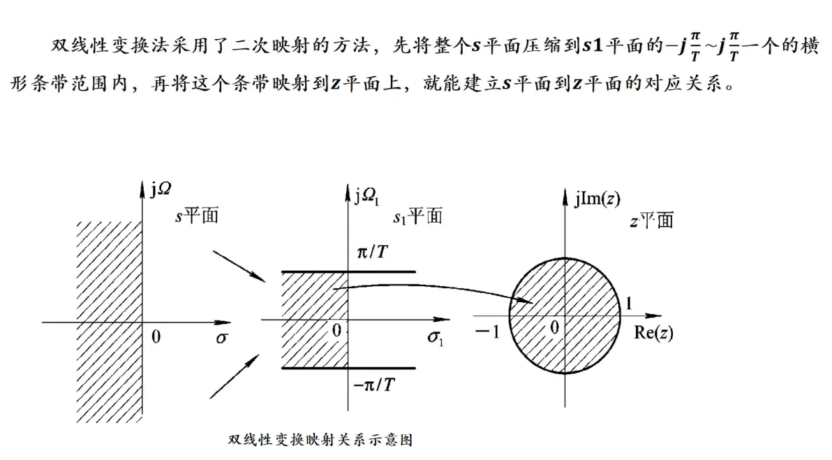
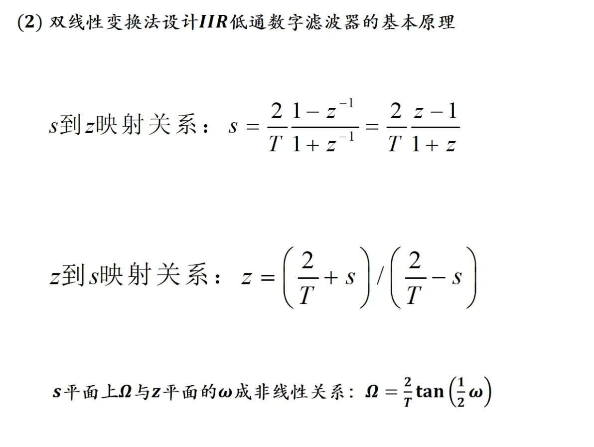
(2) 双线性变换法设计IIR低通数字滤波器的基本原理

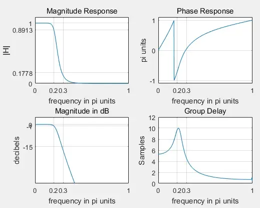
例6：利用巴特沃斯原型低通，采用双线性变换设计一个数字低通，通带截止频率ω_p=0.2π，通带最大衰减α_p=1dB，阻带截止频率ω_s=0.3π，阻带最小衰减α_s=15dB，绘制数字低通的幅频特性、损耗函数、相频特性曲线和群延迟。

wp = 0.2*pi;             % digital Passband freq in Hz

ws = 0.3*pi;             % digital Stopband freq in Hz

Rp = 1;               % Passband ripple in dB

As = 15;               % Stopband attenuation in dB

T = 1;

Fs = 1/T;              % Set T=1

OmegaP = (2/T)*tan(wp/2);      % Prewarp Prototype Passband freq

OmegaS = (2/T)*tan(ws/2);      % Prewarp Prototype Stopband freq

ep = sqrt(10^(Rp/10)-1);       % Passband Ripple parameter

Ripple = sqrt(1/(1+ep*ep));     % Passband Ripple

Attn = 1/(10^(As/20));        % Stopband Attenuation

[cs,ds] = afd_butt(OmegaP,OmegaS,Rp,As);

[b,a] = bilinear(cs,ds,T)

[C,B,A] = dir2cas(b,a)

[db,mag,pha,grd,w] = freqz_m(b,a);

subplot(2,2,1);

plot(w/pi,mag);

grid on

title('Magnitude Response')

xlabel('frequency in pi units');

ylabel('|H|');

axis([0,1,0,1.1])

set(gca,'XTickMode','manual','XTick',[0,0.2,0.3,1]);

set(gca,'YTickmode','manual','YTick',[0,Attn,Ripple,1]);

subplot(2,2,3);

plot(w/pi,db);

grid on

title('Magnitude in dB');

xlabel('frequency in pi units');

ylabel('decibels');

axis([0,1,-40,5]);

set(gca,'XTickMode','manual','XTick',[0,0.2,0.3,1]);

set(gca,'YTickmode','manual','YTick',[-50,-As,-Rp,0]);

subplot(2,2,2);

plot(w/pi,pha/pi);

grid on

title('Phase Response')

xlabel('frequency in pi units');

ylabel('pi units');

axis([0,1,-1.1,1.1]);

set(gca,'XTickMode','manual','XTick',[0,0.2,0.3,1]);

set(gca,'YTickmode','manual','YTick',[-1,0,1]);

subplot(2,2,4);

plot(w/pi,grd);

grid on

title('Group Delay')

xlabel('frequency in pi units');

ylabel('Samples');

axis([0,1,0,12])

set(gca,'XTickMode','manual','XTick',[0,0.2,0.3,1]);

set(gca,'YTickmode','manual','YTick',[0:2:12]);

*** Butterworth Filter Order = 6

b =

 0.0006  0.0035  0.0087  0.0116  0.0087  0.0035  0.0006

a =

 1.0000  -3.3143  4.9501  -4.1433  2.0275  -0.5458  0.0628

C =

 5.7969e-04

B =

 1.0000  2.0191  1.0195

 1.0000  1.9805  0.9809

 1.0000  2.0004  1.0000

A =

 1.0000  -0.9459  0.2342

 1.0000  -1.0541  0.3753

 1.0000  -1.3143  0.7149

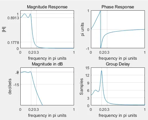
例7：利用切比雪夫I型低通原型，采用双线性变换设计数字低通，通带截止频率ω_p=0.2π，通带最大衰减α_p=1dB，阻带截止频率ω_s=0.3π，阻带最小衰减α_s=15dB，绘制数字低通的幅频、损耗函数、相频特性曲线和群延迟。

clear all;close all;clc;

wp = 0.2*pi;             % digital Passband freq in Hz

ws = 0.3*pi;             % digital Stopband freq in Hz

Rp = 1;               % Passband ripple in dB

As = 15;               % Stopband attenuation in dB

T = 1; Fs = 1/T;           % Set T=1

OmegaP = (2/T)*tan(wp/2);      % Prewarp Prototype Passband freq

OmegaS = (2/T)*tan(ws/2);      % Prewarp Prototype Stopband freq

ep = sqrt(10^(Rp/10)-1);       % Passband Ripple parameter

Ripple = sqrt(1/(1+ep*ep));     % Passband Ripple

Attn = 1/(10^(As/20));        % Stopband Attenuation

[cs,ds] = afd_chb1(OmegaP,OmegaS,Rp,As);

[b,a] = bilinear(cs,ds,T)

[C,B,A] = dir2cas(b,a)

[db,mag,pha,grd,w] = freqz_m(b,a);

subplot(2,2,1);

plot(w/pi,mag);

grid on

title('Magnitude Response')

xlabel('frequency in pi units');

ylabel('|H|');

axis([0,1,0,1.1])

set(gca,'XTickMode','manual','XTick',[0,0.2,0.3,1]);

set(gca,'YTickmode','manual','YTick',[0,Attn,Ripple,1]);

subplot(2,2,3);

plot(w/pi,db);

grid on

title('Magnitude in dB');

xlabel('frequency in pi units');

ylabel('decibels’);

axis([0,1,-40,5]);

set(gca,'XTickMode','manual','XTick',[0,0.2,0.3,1]);

set(gca,'YTickmode','manual','YTick',[-50,-As,-Rp,0]);

subplot(2,2,2);

plot(w/pi,pha/pi);

grid on

title('Phase Response')

xlabel('frequency in pi units');

ylabel('pi units');

axis([0,1,-1,1]);

set(gca,'XTickMode','manual','XTick',[0,0.2,0.3,1]);

set(gca,'YTickmode','manual','YTick',[-1,0,1]);

subplot(2,2,4);

plot(w/pi,grd);

grid on

title('Group Delay')

xlabel('frequency in pi units');

ylabel('Samples');

axis([0,1,0,15])

set(gca,'XTickMode','manual','XTick',[0,0.2,0.3,1]);

set(gca,'YTickmode','manual','YTick',[0:3:15]);

二、实验内容

1、设计一个Butterworth数字低通滤波器，满足如下级数指标：

通带边界频率ω_p=0.4π，通带最大衰减α_p=0.5dB；

阻带边界频率ω_s=0.6π，阻带最小衰减数α_s=50dB。

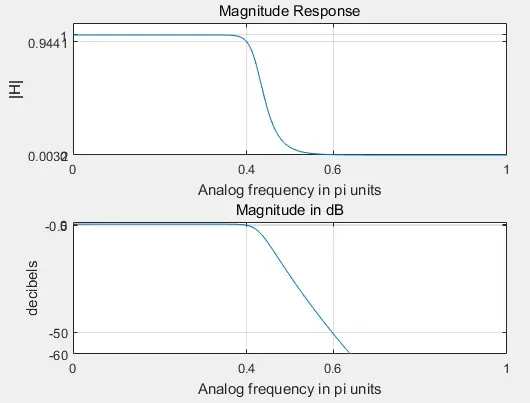
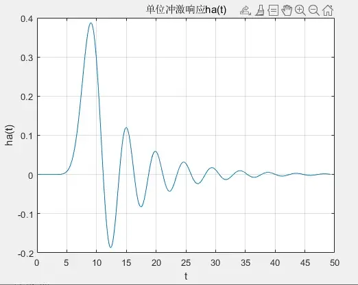
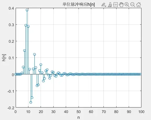
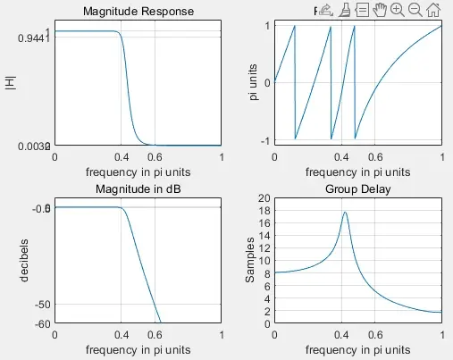
   采用冲激响应不变法，选取 T=1，记录所得的模拟滤波器的阶数N，求出有理函数形式的系统函数，画出模拟滤波器幅频、相频特性曲线和冲激响应h_a(t)，画出数字滤波器的幅频、相频特性曲线和单位脉冲响应h[n]。

sys = tf(B,A);

[ha,t] = impulse(sys); % B，A分别是模拟滤波器系统函数├ H(s)分子、分母多项式系数向量

plot(t,ha);

[hn,n] = impz(b,a,N); %b，a分别是数字滤波器系统函数├ H(z)的分子、分母多项式系数向量

stem(n,hn);

2、设计一个Chebyshev I型数字低通滤波器，满足如下级数指标：

通带边界频率ω_p=0.4π，通带最大衰减α_p=0.5dB；

阻带边界频率ω_s=0.6π，阻带最小衰减数α_s=50dB。

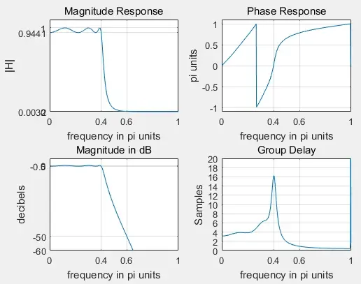
   采用双线性变换法，选取采样周期T=1，记录所得的模拟滤波器的阶数N，求出有理函数形式的系统函数，画出模拟滤波器和数字滤波器的频率响应的幅频和相频特性曲线。

*** Chebyshev-1 Filter Order = 6

b =

 0.0033  0.0196  0.0490  0.0654  0.0490  0.0196  0.0033

a =

 1.0000  -2.6264  4.1118  -4.0835  2.7113  -1.1270  0.2353

C =

 0.0033

B =

 1.0000  2.0118  1.0119

 1.0000  1.9881  0.9882

 1.0000  2.0002  1.0000

A =

 1.0000  -0.5566  0.8635

 1.0000  -0.8502  0.6194

 1.0000  -1.2196  0.4400

免责声明：本文系网络转载或改编，未找到原创作者，版权归原作者所有。如涉及版权，请联系删