scikit-learn不够用？尝试更高级的机器学习扩展库：mlxtend

Author：louwill

    mlxtend是一款高级的机器学习扩展库，可用于日常机器学习任务的主要工具，也可以作为 sklearn  的一个补充和辅助工具。

    mlxtend主要包括以下模块：

• 分类器
• 聚类器
• 数据
• 评估方法
• 特征提取
• 特征选择
• 文件读写
• 关联算法
• 常见概念
• 图像
• 数学
• 绘图
• 预处理
• 回归器
• 文本

    下面分别从分类器、图像、绘图和预处理等几个模块来展示mlxtend的强大功能。

分类器

    mlxtend提供了多种分类和回归算法api，包括多层感知机、stacking分类器、逻辑回归等。以逻辑回归为例：

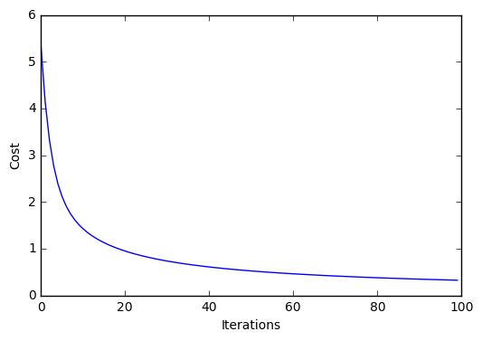
from mlxtend.data import iris_data	from mlxtend.plotting import plot_decision_regions	from mlxtend.classifier import LogisticRegression	import matplotlib.pyplot as plt	 	# Loading Data	 	X, y = iris_data()	X = X[:, [0, 3]] # sepal length and petal width	X = X[0:100] # class 0 and class 1	y = y[0:100] # class 0 and class 1	 	# standardize	X[:,0] = (X[:,0] - X[:,0].mean()) / X[:,0].std()	X[:,1] = (X[:,1] - X[:,1].mean()) / X[:,1].std()	 	lr = LogisticRegression(eta=0.1, 	                        l2_lambda=0.0, 	                        epochs=100,	                        minibatches=1, # for Gradient Descent	                        random_seed=1,	                        print_progress=3)	lr.fit(X, y)	 	plot_decision_regions(X, y, clf=lr)	plt.title('Logistic Regression - Gradient Descent')	plt.show()	 	plt.plot(range(len(lr.cost_)), lr.cost_)	plt.xlabel('Iterations')	plt.ylabel('Cost')	plt.show()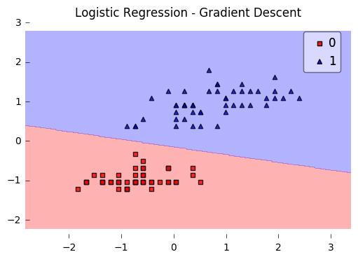

图像

    图像模块提供了人脸特征点提取的api，示例如下：

import imageio	import matplotlib.pyplot as plt	from mlxtend.image import extract_face_landmarks	 	img = imageio.imread('test-face.png')	landmarks = extract_face_landmarks(img)	print(landmarks.shape)	print('\n\nFirst 10 landmarks:\n', landmarks[:10])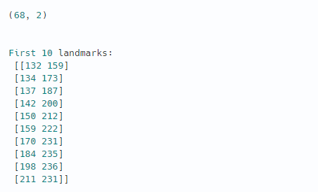

可视化展示：

fig = plt.figure(figsize=(15, 5))	ax = fig.add_subplot(1, 3, 1)	ax.imshow(img)	ax = fig.add_subplot(1, 3, 2)	ax.scatter(landmarks[:, 0], -landmarks[:, 1], alpha=0.8)	ax = fig.add_subplot(1, 3, 3)	img2 = img.copy()	for p in landmarks:	    img2[p[1]-3:p[1]+3,p[0]-3:p[0]+3,:] = (255, 255, 255)	ax.imshow(img2)	plt.show()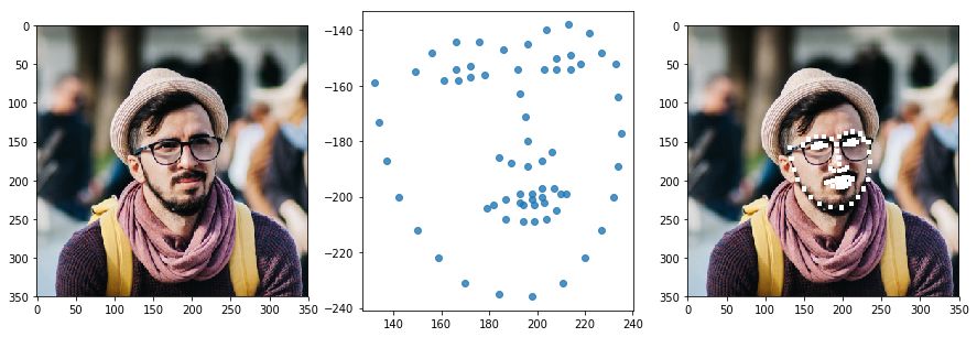

展示人脸特征点：

import numpy as np	import matplotlib.pyplot as plt	 	left = np.array([36, 37, 38, 39, 40, 41])	right = np.array([42, 43, 44, 45, 46, 47])	 	fig = plt.figure(figsize=(10,10))	plt.plot(landmarks[:,0], -landmarks[:,1], 'ro', markersize=8, alpha = 0.5)	for i in range(landmarks.shape[0]):	    plt.text(landmarks[i,0]+1, -landmarks[i,1], str(i), size=14)	 	 	left_eye = np.mean(landmarks[left], axis=0)	right_eye = np.mean(landmarks[right], axis=0)	print('Coordinates of the Left Eye: ', left_eye)	print('Coordinates of the Right Eye: ', right_eye)	plt.plot([left_eye[0]], [-left_eye[1]], 	            marker='+', color='blue', markersize=10, mew=4)	 	plt.plot([right_eye[0]], [-right_eye[1]], 	            marker='+', color='blue', markersize=10, mew=4)	 	plt.xticks([])	plt.yticks([])	plt.show()

Coordinates of the Left Eye:  [169.33333333 156.        ]	Coordinates of the Right Eye:  [210.83333333 152.16666667]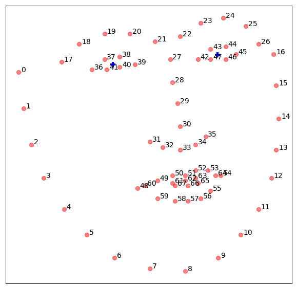

绘图

    mlxtend的绘图模块提供了各种机器学习辅助绘图工具，比如分类散点图、热图、决策边界图、多分类混淆矩阵图等等。以多分类混淆 矩阵  图为例，sklearn的plot_confusion模块只提供了绘制二分类的混淆矩阵图，如果想绘制多分类的混淆矩阵，尝试使用mlxtend的plot_confusion_matrix函数。示例如下：

import matplotlib.pyplot as plt	from mlxtend.evaluate import confusion_matrix	from mlxtend.plotting import plot_confusion_matrix	 	y_target =    [1, 1, 1, 0, 0, 2, 0, 3]	y_predicted = [1, 0, 1, 0, 0, 2, 1, 3]	 	cm = confusion_matrix(y_target=y_target, 	                      y_predicted=y_predicted, 	                      binary=False)	 	fig, ax = plot_confusion_matrix(conf_mat=cm)	plt.show()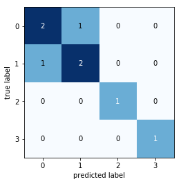

    再来看如何绘制模型的决策边界图。比如我们想看看SVM在 iris数据集 上的分类效果，尝试绘制其决策边界图：

from mlxtend.plotting import plot_decision_regions	import matplotlib.pyplot as plt	from sklearn import datasets	from sklearn.svm import SVC	 	# Loading some example data	iris = datasets.load_iris()	X = iris.data[:, [0, 2]]	y = iris.target	 	# Training a classifier	svm = SVC(C=0.5, kernel='linear')	svm.fit(X, y)	 	 	# Plotting decision regions	plot_decision_regions(X, y, clf=svm, legend=2)	 	# Adding axes annotations	plt.xlabel('sepal length [cm]')	plt.ylabel('petal length [cm]')	plt.title('SVM on Iris')	plt.show()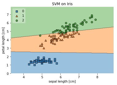

预处理

    mlxtend预处理模块提供了各种数据标准化和归一化方法，这里以分类变量的one-hot编码为例。mlxtend下的one_hot可对列表或numpy数组的数据进行转换：

from mlxtend.preprocessing import one_hot	import numpy as np	# numpy array	y = np.array([0, 1, 2, 1, 2])	one_hot(y)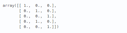

from mlxtend.preprocessing import one_hot	# list	y = [0, 1, 2, 1, 2]	one_hot(y)

mlxtend其他模块和更多功能参考官方文档：

http://rasbt.github.io/mlxtend/

GitHub源码地址：

https://github.com/rasbt/mlxtend

参考资料：

http://rasbt.github.io/mlxtend/user_guide

免责声明：本文系网络转载或改编，未找到原创作者，版权归原作者所有。如涉及版权，请联系删