


软件

产品


龙格库塔方法原理
隐式Adams原理: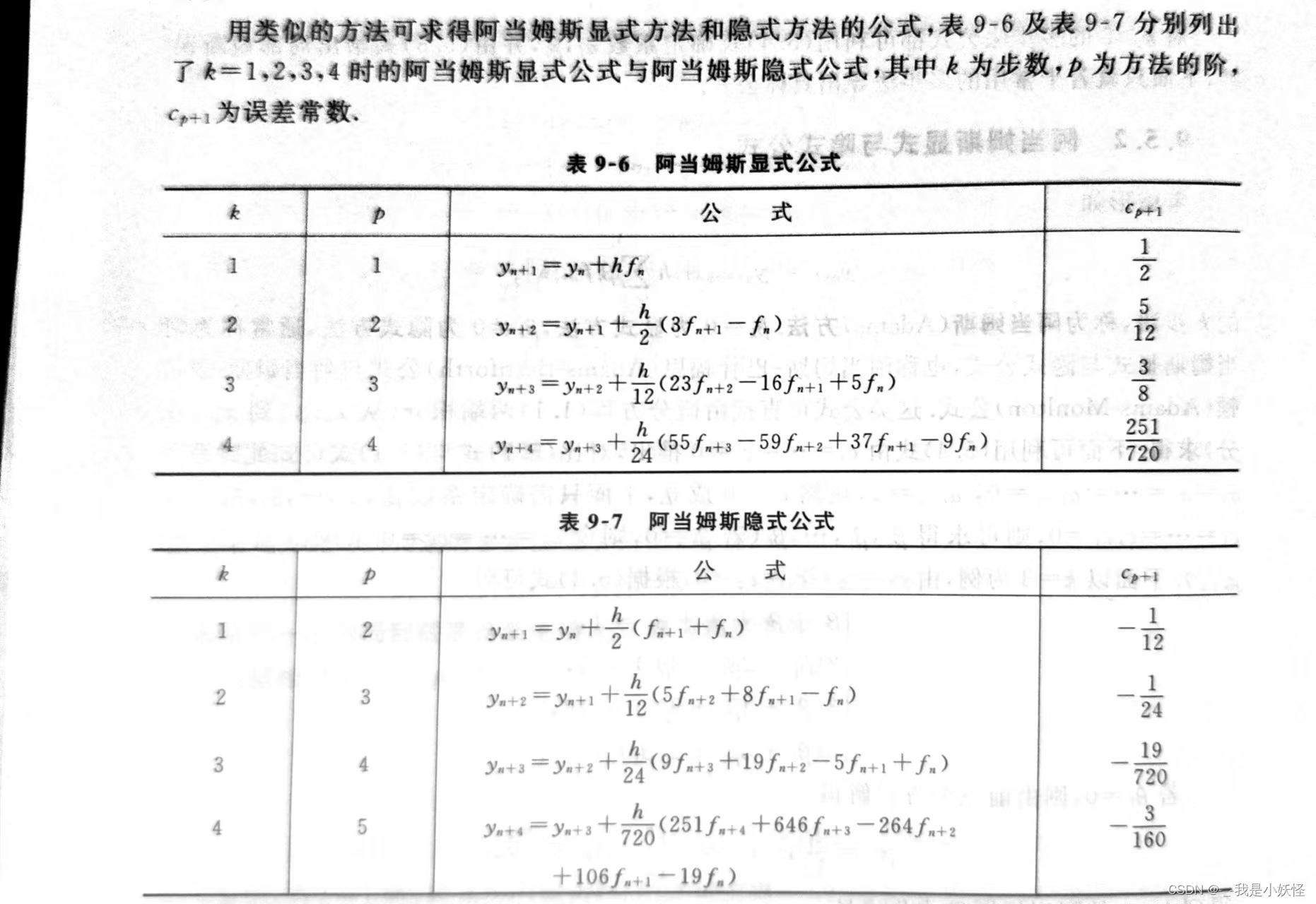
# Code   : UTF-8
# Author : CSDNwoShiXiaoYaoGuai_zhz
# Date   : 2023/11/20
# Project: 4阶Runge-Kutta方法解常微分方程通用程序

def rungeKutta4oneStep(h:float, x0:float, y0:float, f)->float:
    '''
        四阶龙格库塔方法单步
        ------------------------------------------------------------------------
        h   Input   积分步长
        x0  Input   自变量
        y0  Input   x0处对应的因变量
        f   Input   常微分方程
        ------------------------------------------------------------------------
        Return: x0+h处对应的因变量
    '''
    k1 = h * f(x0, y0) * 1.0
    k2 = h * f(x0 + 0.5 * h, y0 + 0.5 * k1) * 1.0
    k3 = h * f(x0 + 0.5 * h, y0 + 0.5 * k2) * 1.0
    k4 = h * f(x0 + h, y0 + k3) * 1.0
    return y0 + (k1 + 2 * k2 + 2 * k3 + k4) / 6.0

def rungeKutta4(h:float, x0:float, y0:float, x:float, f)->list:
    '''
        四阶龙格库塔方法
        ------------------------------------------------------------------------
        h   Input   积分步长
        x0  Input   初始自变量
        y0  Input   x0处对应的因变量 (初始条件)
        x   Input   待求解处相应的自变量
        f   Input   常微分方程
        ------------------------------------------------------------------------
        Return: [[x0, x1, ..., xn], [y0, y1, ..., yn]]
    '''
    steps = int(((x - x0) / h) + 0.5)
    xs = []
    ys = []
    for i in range(0, steps + 1):
        xi = x0 + i * h
        if i == 0:
            yi = y0
        else:
            yi = yi1
        yi1 = rungeKutta4oneStep(h, xi, yi, f)
        xs.append(xi)
        ys.append(yi)
    return [xs, ys]
# Code   : UTF-8
# Author : CSDNwoShiXiaoYaoGuai_zhz
# Date   : 2023/11/20
# Project: Adams隐式3阶方法解常微分方程通用程序

import rungeKutta as rk

def adams3Explicit(h:float, y0s:list, fs:list)->float:
    '''
        显式三阶Adams方法
        ------------------------------------------------------------------------
        h   Input   积分步长
        y0s Input   [y_n, y_(n+1)]
        fs  Input   [f(x_n, y_n), f(x_(n+1), y_(n+1))]
        ------------------------------------------------------------------------
        Return: y_(n+2)
    '''
    return y0s[-1] + h * (3 * fs[-1] - fs[-2]) / 2.0

def adams3oneStep(h:float, x0s:list, y0s:list, f)->float:
    '''
        隐式三阶Adams方法单步
        ------------------------------------------------------------------------
        h   Input   积分步长
        x0s Input   [x_n, x_(n+1)]
        y0s Input   [y_n, y_(n+1)]
        f   Input   常微分方程
        ------------------------------------------------------------------------
        Return: y_(n+2)
    '''
    fs = []
    for i in range(len(x0s)):
        fs.append(f(x0s[i], y0s[i]))
    y0 = rk.rungeKutta4oneStep(h, x0s[-1], y0s[-1], f) # 龙格库塔方法提供初值
    # y0 = adams3Explicit(h, y0s, fs) # Adams显式3阶方法提供初值
    # y0 = 10 # 任意常数提供初值

    # 开始迭代
    iter = 0
    changeFactor = 100
    while ((iter < 100) and (changeFactor > 1e-12)):
        fn2 = f(x0s[-1] + h, y0)
        yk = y0s[-1] + h * (5 * fn2 + 8 * fs[-1] - fs[-2]) / 12.0
        changeFactor = abs((yk - y0))
        # changeFactor = abs((yk - y0) / y0)
        iter = iter + 1
        y0 = yk
    return y0

def adams3(h, x0, y0, x, f)->list:
    '''
        隐式三阶Adams方法
        ------------------------------------------------------------------------
        h   Input   积分步长
        x0  Input   初始自变量
        y0  Input   x0处对应的因变量 (初始条件)
        x   Input   待求解处相应的自变量
        f   Input   常微分方程
        ------------------------------------------------------------------------
        Return: [[x0, x1, ..., xn], [y0, y1, ..., yn]]
    '''
    [xs, ys] = rk.rungeKutta4(h, x0, y0, x0 + h, f)
    steps = int(((x - x0) / h) + 0.5)

    for i in range(0, steps - 1):
        y = adams3oneStep(h, xs[-2:], ys[-2:], f)
        xs.append(xs[-1] + h)
        ys.append(y)
    return [xs, ys]
# Code   : UTF-8
# Author : CSDNwoShiXiaoYaoGuai_zhz
# Date   : 2023/11/20
# Project: 结果绘制

import matplotlib.pyplot as plt

def drawResult1(h, rkX, rkY, adamsX, adamsY, diffRk, diffAdams):
    fig = plt.figure(dpi = 200)
    ax1 = plt.subplot(221)
    ax1.plot(rkX, rkY, 'o', label='RK4')
    ax2 = plt.subplot(222)
    ax2.plot(adamsX, adamsY, '+', label='AD3', color = 'orange')
    ax3 = plt.subplot(223)
    ax3.plot(diffRk[0], diffRk[1], 'o', label='biaRK4')
    ax4 = plt.subplot(224)
    ax4.plot(diffAdams[0], diffAdams[1], '+', label='biaAD3', color = 'orange')

    for ax in [ax1, ax2, ax3, ax4]:
        ax.set_xlim(-0.1, 1.6)
        ax.legend(ncol=1)
        ax.grid()
        ax.set_title('Step length: ' + str(h))
        ax.set_xlabel('x')
        ax.set_ylabel('y')
    plt.tight_layout()
    plt.savefig('StepLength' + str(h) + '.jpg')

def drawResult2(lnhs, lnRkErrors, lnAdErrors, kRk, kAd):
    fig, ax = plt.subplots()
    ax.plot(lnhs, lnRkErrors, 'o--', label = 'RK, k=' + str(kRk))
    ax.plot(lnhs, lnAdErrors, 's--', label = 'Adams, k=' + str(kAd))
    ax.legend()
    ax.set_xlabel('ln(h)')
    ax.set_ylabel('ln(error)')
    plt.grid()
    plt.tight_layout()
    plt.savefig('RelationLnhAndLnerror.jpg', dpi = 250)
# Code   : UTF-8
# Author : CSDNwoShiXiaoYaoGuai_zhz
# Date   : 2023/11/20
# Project: 主程序

import rungeKutta as rk
import adams as ad
import drawChart as dc
import math
import numpy as np

def calDiff(xs:list, ys:list, fExact)->list:
    '''
        计算数值解相对于精确解的差
        ------------------------------------------------------------------------
        xs      Input   自变量序列
        ys      Input   自变量对应的因变量数值解序列
        fExact  Input   因变量关于自变量的精确解函数
        ------------------------------------------------------------------------
        Return: [[x0, x1, ..., xn], [diff0, diff1, ..., diffn]]
    '''
    diffs = []
    for i in range(len(xs)):
        diff = ys[i] - fExact(xs[i])
        diffs.append(diff)
    return [xs, diffs]

def differentialEquation(x, y):
    ''' 用户自定义的常微分方程 '''
    return (-1) * (x ** 2) * (y ** 2)

def solExact(x):
    ''' 用户自定义的常微分方程精确解 '''
    return 3.0 / (1 + x ** 3)

def lsq(x, l):
    b = []
    for i in range(len(x)):
        b.append([x[i], 1])
    b = np.mat(b)

    l = np.mat(l).T
    x = np.linalg.inv(b.T * b) * b.T * l
    return np.array(x)[0][0]


if __name__ == '__main__':
    hs = []
    rkErrors = []
    adErrors = []

    with open('Result.txt', 'w', encoding='utf-8') as f:
        f.write('步长\t4阶RK数值解\t\tRK数值解与精确解差值\t\t' +
        '隐式3阶Adams数值解\t隐式3阶Adams数值解与精确解差值\n')
    print('步长\t4阶RK数值解\t\tRK数值解与精确解差值\t\t' +
        '隐式3阶Adams数值解\t隐式3阶Adams数值解与精确解差值')
    for h in [0.1, 0.1 / 2, 0.1 / 4, 0.1 / 8]:
        # RK方法
        [rkX,rkY] = rk.rungeKutta4(h, 0, 3, 1.5, differentialEquation)
        # Adams方法
        [adamsX,adamsY] = ad.adams3(h, 0, 3, 1.5, differentialEquation)

        # RK数值解与精确解的差值
        diffRk = calDiff(rkX, rkY, solExact)
        # Adams数值解与精确解的差值
        diffAdams = calDiff(adamsX, adamsY, solExact)

        hs.append(math.log(h, math.e)) # ln(h)
        rkErrors.append(math.log(abs(diffRk[1][-1]), math.e)) # ln(err) by RK
        adErrors.append(math.log(abs(diffAdams[1][-1]), math.e)) # ln(err) by AD

        # 结果输出
        print(str(h) + '\t' + str(rkY[-1]) + '\t' + str(diffRk[1][-1]) + '\t\t'
            + str(adamsY[-1]) + '\t' + str(diffAdams[1][-1]))
        with open('Result.txt', 'a') as f:
            f.write(str(h) + '\t' + str(rkY[-1]) + '\t' + str(diffRk[1][-1])
            + '\t\t' + str(adamsY[-1]) + '\t' + str(diffAdams[1][-1]) + '\n')

        # 结果1绘制
        dc.drawResult1(h, rkX, rkY, adamsX, adamsY, diffRk, diffAdams)

    # 计算回归系数
    kRk = lsq(hs, rkErrors)
    kAd = lsq(hs, adErrors)

    # 结果2绘制
    dc.drawResult2(hs, rkErrors, adErrors, kRk, kAd)
不同步长时结果
步长为0.1时两种方法的结果(上图)以及 数值解 与精确解的差值(下图)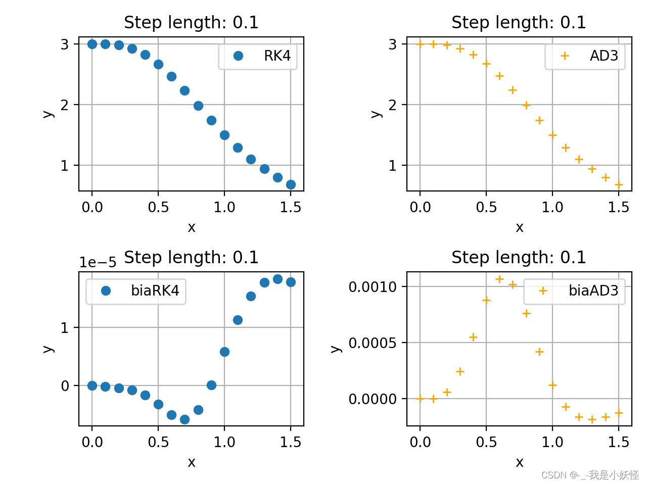
两种方法的数值解与精确解的差值的ln值与步长ln值关系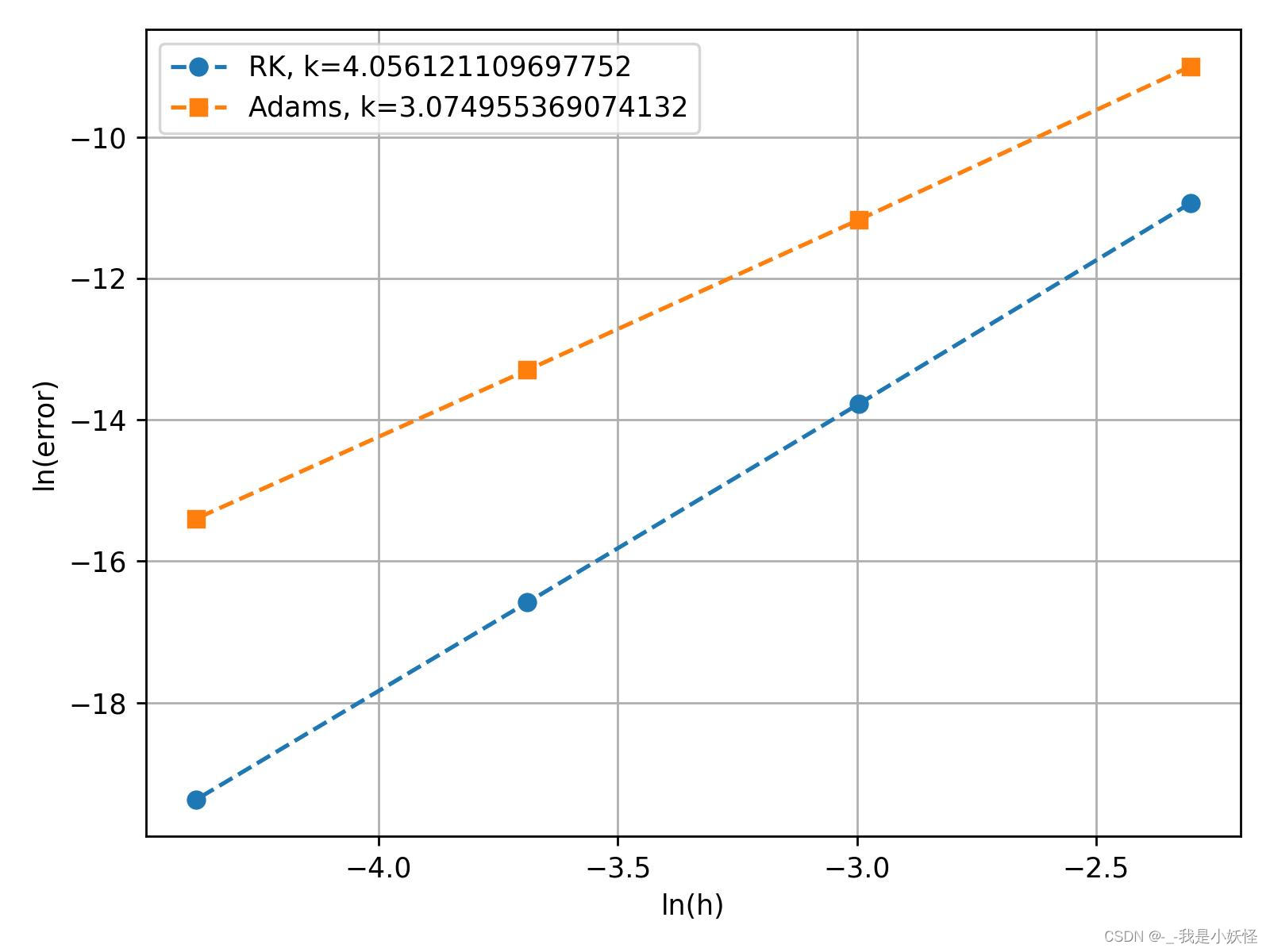
免责声明:本文系网络转载或改编,未找到原创作者,版权归原作者所有。如涉及版权,请联系删
 技术文档
技术文档
 推荐好文
推荐好文


 155-2731-8020


