Matlab地震振幅属性分析：洛马普列塔地震数据实例

加载地震数据

文件 quake.mat 包含圣克鲁斯山脉在 1989 年 10 月 17 日发生的洛马普列塔地震的 200Hz 数据。该数据由加州大学圣克鲁斯分校的 Joel Yellin 通过 Charles F. Richter 地震实验室提供。

首先加载数据。

load quake

whos e n v

Name Size Bytes Class Attributes

e 10001x1 80008 double

n 10001x1 80008 double

v 10001x1 80008 double

工作区中有三个变量，包含由位于加州大学圣克鲁斯分校的自然科学大楼的一个加速计记录的时间跟踪。加速计记录了地震波的主震幅值。变量 n、e、v 指代该工具测量的三个定向分量，工具已调整为与断层平行，其 N 方向指向萨克拉门托方向。数据未针对工具响应进行纠正。

创建一个变量 Time，其中包含以 200Hz 采样的时间戳，并且长度与其他向量相同。使用 seconds 函数和乘法表示正确的单位以实现该 Hz (s−1) 采样率。这将生成一个适用于表示已用时间的 duration 变量。

Time = (1/200)*seconds(1:length(e))';

whos Time

Name Size Bytes Class Attributes

Time 10001x1 80010 duration

组织时间表中的数据

可以将这些单独的变量放到 table 或 timetable 中，以便于使用。timetable 提供了灵活丰富的时间戳数据处理功能。使用时间和三个加速度变量创建 timetable，并提供更有意义的变量名称。使用 head 函数来显示前八行。

varNames = {'EastWest', 'NorthSouth', 'Vertical'};

quakeData = timetable(Time, e, n, v, 'VariableNames', varNames);

head(quakeData)

ans=8×3 timetable

Time EastWest NorthSouth Vertical

_________ ________ __________ ________

0.005 sec 5 3 0

0.01 sec 5 3 0

0.015 sec 5 2 0

0.02 sec 5 2 0

0.025 sec 5 2 0

0.03 sec 5 2 0

0.035 sec 5 1 0

0.04 sec 5 1 0

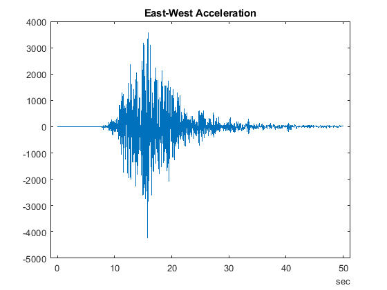
通过使用圆点下标访问 timetable 中的变量来探查数据。(有关圆点下标的详细信息，请参阅访问表中的数据。)我们选择了“东-西”振幅并将其作为持续时间的函数来执行 plot 操作。

plot(quakeData.Time,quakeData.EastWest)

title('East-West Acceleration')

缩放数据

按照重力加速度缩放数据或者将表中的每个变量与常量相乘。由于这些变量都具有相同类型 (double)，因此可以使用维度名称 Variables 访问所有变量。请注意，quakeData.Variables 提供了一种直接修改时间表中数值的方式。

quakeData.Variables = 0.098*quakeData.Variables;

选择要探查的数据子集

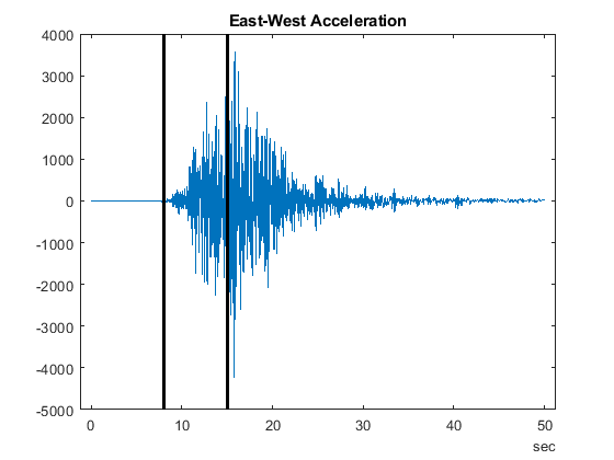
我们对冲击波幅值从几乎为零增大到最大水平的时间区域感兴趣。直接观察上图可看到，从 8 至 15 秒这个时间段是我们需要关注的。为了显示更清晰，我们在选定的时间点绘制黑色线条以引起对该时间段的关注。所有后续计算都将涉及此时间段。

t1 = seconds(8)*[1;1];

t2 = seconds(15)*[1;1];

hold on

plot([t1 t2],ylim,'k','LineWidth',2)

hold off

存储相关数据

使用此区间中的数据创建另一个 timetable。使用 timerange 选择感兴趣的行。

tr = timerange(seconds(8),seconds(15));

dataOfInterest = quakeData(tr,:);

head(dataOfInterest)

ans=8×3 timetable

Time EastWest NorthSouth Vertical

_________ ________ __________ ________

8 sec -0.098 2.254 5.88

8.005 sec 0 2.254 3.332

8.01 sec -2.058 2.352 -0.392

8.015 sec -4.018 2.352 -4.116

8.02 sec -6.076 2.45 -7.742

8.025 sec -8.036 2.548 -11.466

8.03 sec -10.094 2.548 -9.8

8.035 sec -8.232 2.646 -8.134

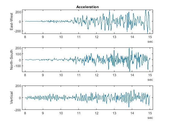
在单独的坐标区上以可视方式呈现三个加速度变量。

figure

subplot(3,1,1)

plot(dataOfInterest.Time,dataOfInterest.EastWest)

ylabel('East-West')

title('Acceleration')

subplot(3,1,2)

plot(dataOfInterest.Time,dataOfInterest.NorthSouth)

ylabel('North-South')

subplot(3,1,3)

plot(dataOfInterest.Time,dataOfInterest.Vertical)

ylabel('Vertical')

计算汇总统计量

我们使用 summary 函数显示有关数据的统计信息。

summary(dataOfInterest)

RowTimes:

Time: 1400x1 duration

Values:

Min 8 sec

Median 11.498 sec

Max 14.995 sec

TimeStep 0.005 sec

Variables:

EastWest: 1400x1 double

Values:

Min -255.09

Median -0.098

Max 244.51

NorthSouth: 1400x1 double

Values:

Min -198.55

Median 1.078

Max 204.33

Vertical: 1400x1 double

Values:

Min -157.88

Median 0.98

Max 134.46

可以使用 varfun 计算其他数据统计信息。在对表或时间表中的每个变量应用函数时，这会非常有用。要应用的函数将以函数句柄的形式传递到 varfun。下面我们将 mean 函数应用于全部三个变量并以表格式输出结果，因为在计算了时间均值之后，时间会变得没有意义。

mn = varfun(@mean,dataOfInterest,'OutputFormat','table')

mn=1×3 table

mean_EastWest mean_NorthSouth mean_Vertical

_____________ _______________ _____________

0.9338 -0.10276 -0.52542

计算速度和位置

为了确定冲击波的传播速度，我们对加速度进行一次积分。我们使用沿时间变量的累积和来获取波前速度。

edot = (1/200)*cumsum(dataOfInterest.EastWest);

edot = edot - mean(edot);

下面我们对全部三个变量执行积分来计算该速度。可以方便地创建函数，并使用 varfun 将该函数应用于 timetable 中的变量。在本例中，我们在文件末尾处包括了该函数，并将其命名为 velFun。

vel = varfun(@velFun,dataOfInterest);

head(vel)

ans=8×3 timetable

Time velFun_EastWest velFun_NorthSouth velFun_Vertical

_________ _______________ _________________ _______________

8 sec -0.56831 0.44642 1.8173

8.005 sec -0.56831 0.45769 1.834

8.01 sec -0.5786 0.46945 1.832

8.015 sec -0.59869 0.48121 1.8114

8.02 sec -0.62907 0.49346 1.7727

8.025 sec -0.66925 0.5062 1.7154

8.03 sec -0.71972 0.51894 1.6664

8.035 sec -0.76088 0.53217 1.6257

将同一函数 velFun 应用于速度以确定位置。

pos = varfun(@velFun,vel);

head(pos)

ans=8×3 timetable

Time velFun_velFun_EastWest velFun_velFun_NorthSouth velFun_velFun_Vertical

_________ ______________________ ________________________ ______________________

8 sec 2.1189 -2.1793 -3.0821

8.005 sec 2.1161 -2.177 -3.0729

8.01 sec 2.1132 -2.1746 -3.0638

8.015 sec 2.1102 -2.1722 -3.0547

8.02 sec 2.107 -2.1698 -3.0458

8.025 sec 2.1037 -2.1672 -3.0373

8.03 sec 2.1001 -2.1646 -3.0289

8.035 sec 2.0963 -2.162 -3.0208

请注意 varfun 所创建的时间表中的变量名称是如何包含所使用函数的名称的。此方法有助于跟踪已对原始数据执行了哪些运算。使用圆点表示法将变量名称重新调整回其原始值。

pos.Properties.VariableNames = varNames;

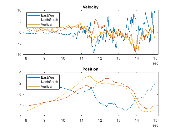
下面我们分别绘制所关注时间段内速度和位置的 3 个分量。

figure

subplot(2,1,1)

plot(vel.Time,vel.Variables)

legend(quakeData.Properties.VariableNames,'Location','NorthWest')

title('Velocity')

subplot(2,1,2)

plot(vel.Time,pos.Variables)

legend(quakeData.Properties.VariableNames,'Location','NorthWest')

title('Position')

以可视方式呈现轨迹

可使用分量值绘制二维或三维轨迹。下面显示了以可视方式呈现这些数据的不同方式。

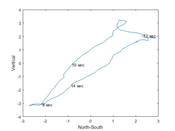
首先使用二维投影。下面是第一张标注有几个时间值的图。

figure

plot(pos.NorthSouth,pos.Vertical)

xlabel('North-South')

ylabel('Vertical')

% Select locations and label

nt = ceil((max(pos.Time) - min(pos.Time))/6);

idx = find(fix(pos.Time/nt) == (pos.Time/nt))';

text(pos.NorthSouth(idx),pos.Vertical(idx),char(pos.Time(idx)))

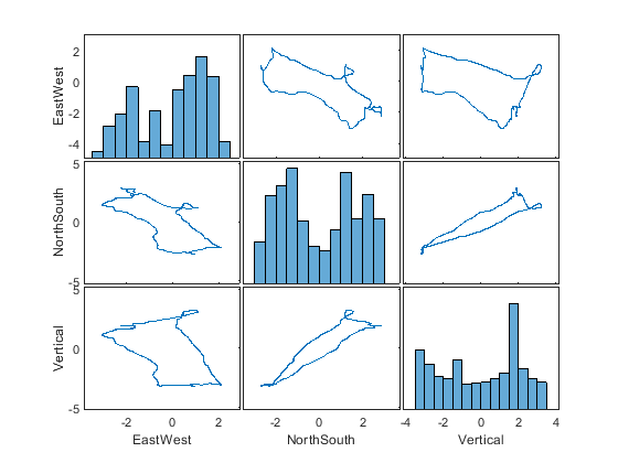
使用 plotmatrix 以可视方式呈现一个网格，其中包含每个变量相对另一变量的散点图，对角线上则是每个变量自身的直方图。输出变量 Ax 表示网格中的每个坐标区，可用于确定要使用 xlabel 和 ylabel 标记的坐标区。

figure

[S,Ax] = plotmatrix(pos.Variables);

for ii = 1:length(varNames)

xlabel(Ax(end,ii),varNames{ii})

ylabel(Ax(ii,1),varNames{ii})

end

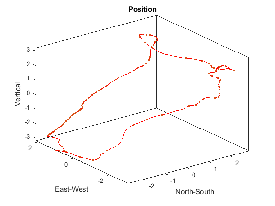
绘制轨迹的三维视图并每隔十个位置点绘制一个圆点。点之间的间距即表示速度。

step = 10;

figure

plot3(pos.NorthSouth,pos.EastWest,pos.Vertical,'r')

hold on

plot3(pos.NorthSouth(1:step:end),pos.EastWest(1:step:end),pos.Vertical(1:step:end),'.')

hold off

box on

axis tight

xlabel('North-South')

ylabel('East-West')

zlabel('Vertical')

title('Position')

支持函数

下面定义了这些函数。

function y = velFun(x)

y = (1/200)*cumsum(x);

y = y - mean(y);

end

免责声明：本文系网络转载或改编，未找到原创作者，版权归原作者所有。如涉及版权，请联系删