超轻量级UNet变种EGeUnet：参数量仅50KB，计算量降低494倍和160倍——医疗图像分割实践

今天看到一篇挺有意思的文章，做的是跟医疗图像分割相关的工作，但是不像之前看到的一些工作一味地去追求高精度，因为医疗领域本身就是一个相对特殊的行业，对于模型产生的结果的精确性要求是很高的，带来的是参数量级的庞大，之所以觉得这篇论文挺有意思的就是因为这里的主要的点在于超轻量级但是并没有导致精度大幅下降。

官方论文地址在这里，如下所示：

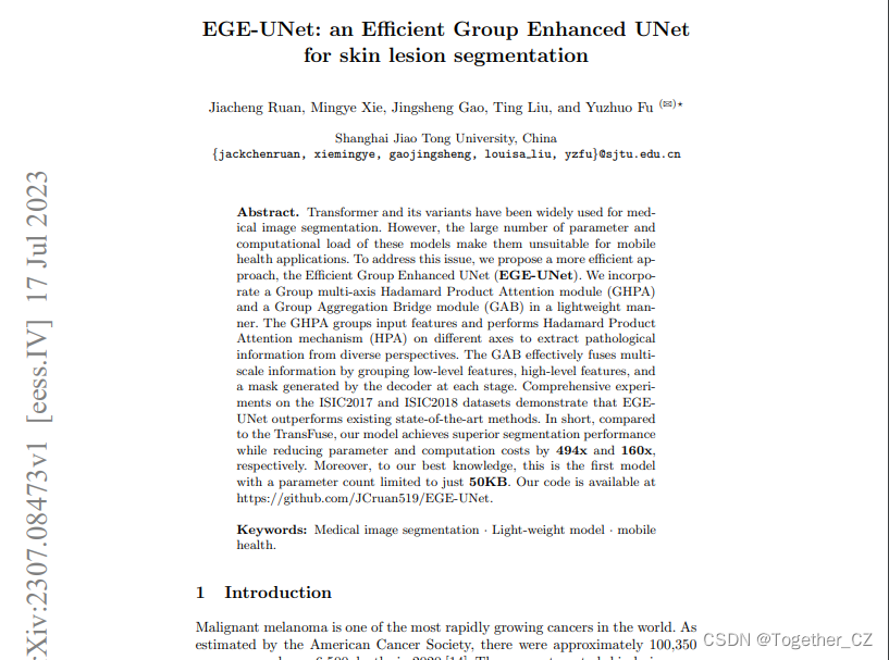
可见刚发表不久。

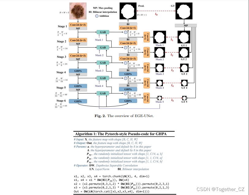
EGE-UNet融合了两个主要模块：

   Group multi-axis Hadamard Product Attention module   (GHPA)

   Group Aggregation Bridge module (GAB)

   GHPA 利用哈达玛积 注意力机制 （HPA），通过将输入特征进行分组，对不同轴进行 HPA 操作，从多个视角提取病变信息。

   GAB 通过分组聚合将不同规模的高级语义特征和低级细节特征以及解码器生成的掩码进行融合，从而有效提取多尺度信息，

   通过融合上述两个模块提出了EGE-UNet模型实现了在参数和计算复杂度极低的情况下优秀的分割性能。

   EGE-UNet的设计沿用了 U 形架构，包括对称的编码器-解码器部分。编码器由六个 stage 组成，各阶段的通道数量为{8, 16, 24, 32, 48, 64}。前三个阶段采用了普通卷积，而后三个阶段使用提出的 GHPA 来从多视角提取表征信息。

   EGE-UNet 在编码器和解码器之间的每个阶段都集成了GAB。此外，模型还利用深监督生成不同规模的掩膜预测，这些预测用于损失函数并作为 GAB 的输入之一。通过这些高级模块的集成，EGE-UNet 在比先前的方法提升了分割性能的同时，显著减少了参数和计算负载。

进一步详情可以自行研读发表的论文。

这里我也是初步了解了一下，主要是想要实际使用一下这个超轻量级的网络，因为我觉得这种类型的网络在现实工作里的意义更大，大参数量高精度模型固然很好，但是并未所有的工业或者是医疗场景里面的设备都具备那么高的算力能够支撑如此庞大的计算量的，如果能在高度轻量化的网络基础上保持不俗的精度性能的话着实还是很有实际意义的。

官方同时开源了项目，地址在这里，如下所示：

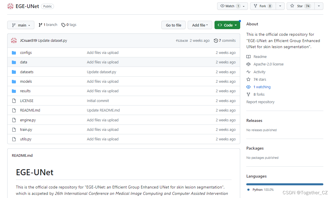
感觉目前的star量很少，估计是了解到的人还不多吧，就让我来带一波热度吧。

从readme来看，作者给出来的实操训练手册可以说是简单到了极致了：

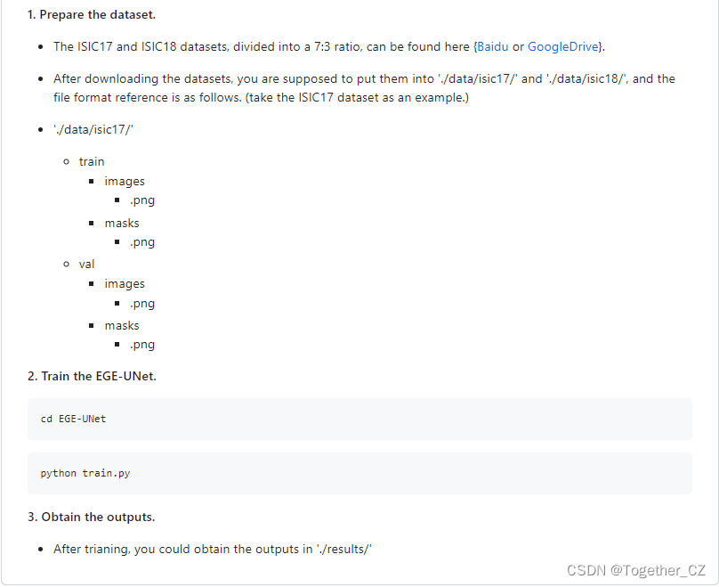
数据集也一并准备好了，地址在这里，如下所示：

自行下载下来即可，体积不大，下载起来应该还是很快的。

下载下载放到项目data目录下面解压缩即可，如下所示：

可以看到：作者同时提供了两组数据集，项目源码默认使用的是isic2017的数据集的。

直接终端执行train.py模块即可，如下所示：

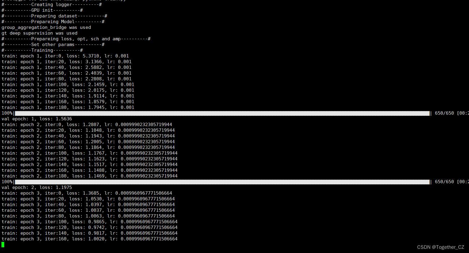
默认300个epoch的迭代计算：

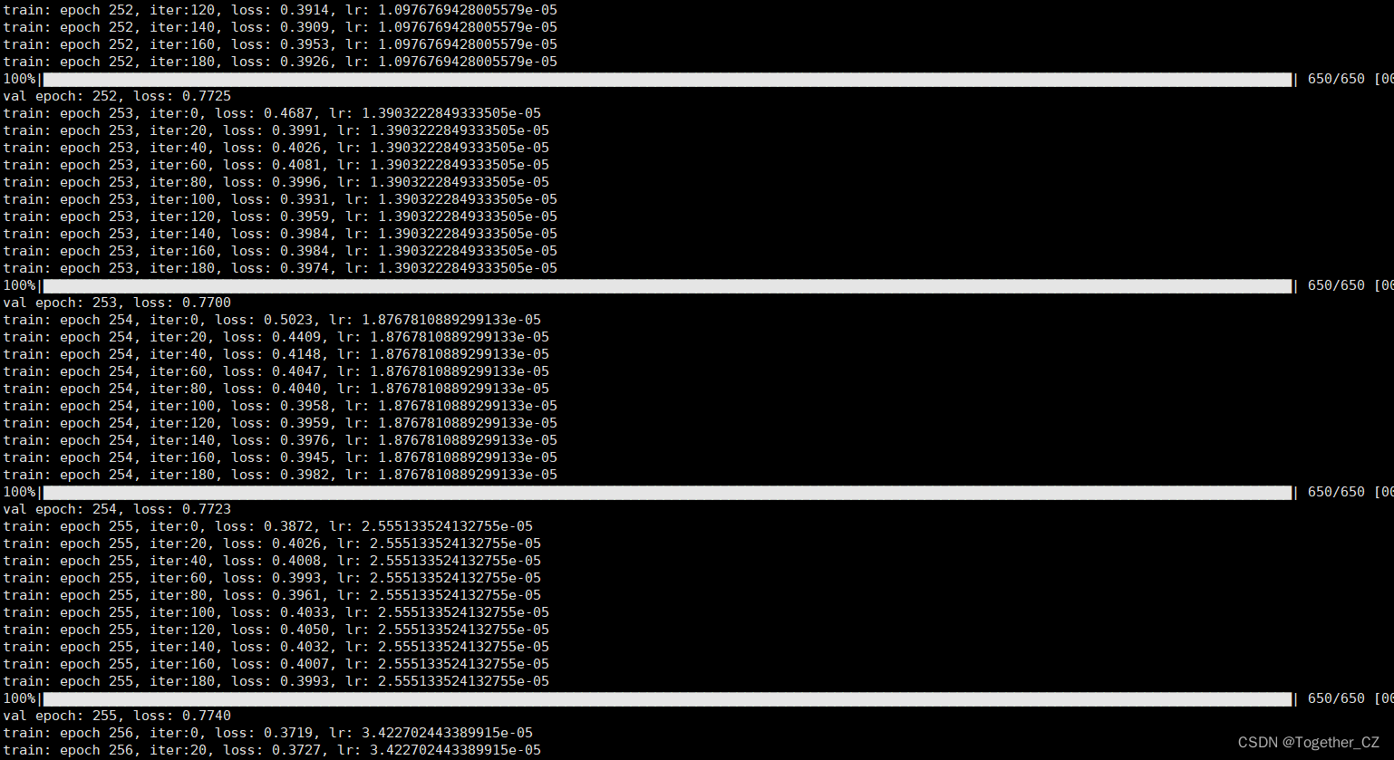
训练完成截图如下所示：

结果默认存储在results目录下。如下所示：

checkpoints目录下存放的是训练得到的模型文件，如下所示：

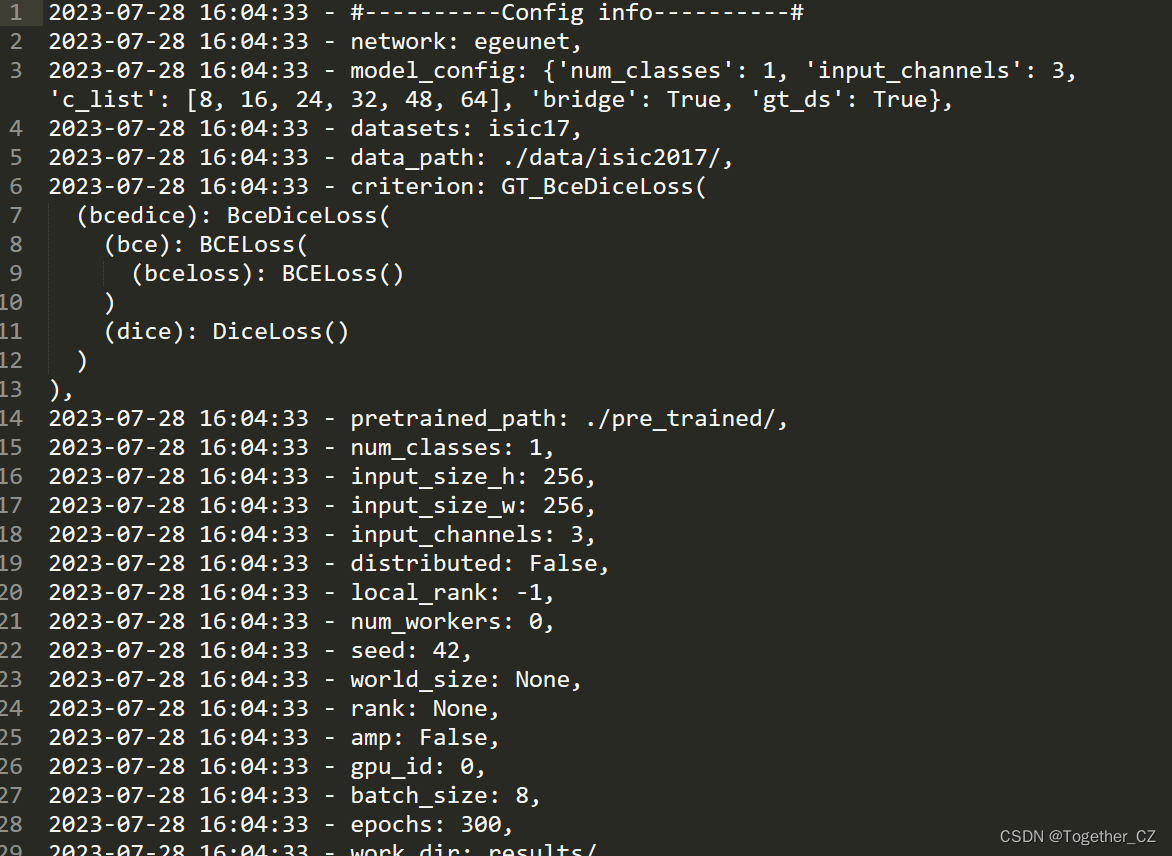
log目录下存放的是训练日志数据，如下所示：

outputs目录下存放的是实际测试的实例图像 可视化  结果，如下所示：

官方项目只提供了训练、评估使用的代码，没有提供离线 推理  可直接使用的代码，但是基于训练和评估部分的代码可以自行开发离线推理的代码，这里我为了能够更加简单的使用开发了专用的可视化系统界面，实例推理效果如下所示：

到这里基本完整的实践就结束了，前面也说过了源码默认使用的是isic2017的数据集，所以后面我又考虑基于isic2018的数据集也开发训练一下模型，只需要修改configs目录下的参数即可，如下所示：

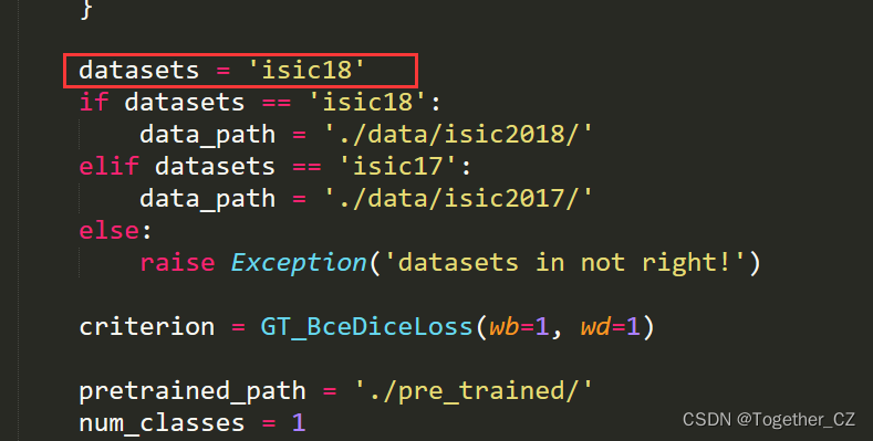
修改后的config_setting模块如下所示：

from torchvision import transformsfrom utils import * from datetime import datetime class setting_config:    """ the config of training setting. """     network = 'egeunet'    model_config = {        'num_classes': 1,         'input_channels': 3,         'c_list': [8,16,24,32,48,64],         'bridge': True,        'gt_ds': True,    }     datasets = 'isic18'     if datasets == 'isic18':        data_path = './data/isic2018/'    elif datasets == 'isic17':        data_path = './data/isic2017/'    else:        raise Exception('datasets in not right!')     criterion = GT_BceDiceLoss(wb=1, wd=1)     pretrained_path = './pre_trained/'    num_classes = 1    input_size_h = 256    input_size_w = 256    input_channels = 3    distributed = False    local_rank = -1    num_workers = 0    seed = 42    world_size = None    rank = None    amp = False    gpu_id = '0'    batch_size = 8    epochs = 300     work_dir = 'results/' + network + '_' + datasets + '_' + datetime.now().strftime('%A_%d_%B_%Y_%Hh_%Mm_%Ss') + '/'     print_interval = 20    val_interval = 30    save_interval = 100    threshold = 0.5     train_transformer = transforms.Compose([        myNormalize(datasets, train=True),        myToTensor(),        myRandomHorizontalFlip(p=0.5),        myRandomVerticalFlip(p=0.5),        myRandomRotation(p=0.5, degree=[0, 360]),        myResize(input_size_h, input_size_w)    ])    test_transformer = transforms.Compose([        myNormalize(datasets, train=False),        myToTensor(),        myResize(input_size_h, input_size_w)    ])     opt = 'AdamW'    assert opt in ['Adadelta', 'Adagrad', 'Adam', 'AdamW', 'Adamax', 'ASGD', 'RMSprop', 'Rprop', 'SGD'], 'Unsupported optimizer!'    if opt == 'Adadelta':        lr = 0.01 # default: 1.0 – coefficient that scale delta before it is applied to the parameters        rho = 0.9 # default: 0.9 – coefficient used for computing a running average of squared gradients        eps = 1e-6 # default: 1e-6 – term added to the denominator to improve numerical stability         weight_decay = 0.05 # default: 0 – weight decay (L2 penalty)     elif opt == 'Adagrad':        lr = 0.01 # default: 0.01 – learning rate        lr_decay = 0 # default: 0 – learning rate decay        eps = 1e-10 # default: 1e-10 – term added to the denominator to improve numerical stability        weight_decay = 0.05 # default: 0 – weight decay (L2 penalty)    elif opt == 'Adam':        lr = 0.001 # default: 1e-3 – learning rate        betas = (0.9, 0.999) # default: (0.9, 0.999) – coefficients used for computing running averages of gradient and its square        eps = 1e-8 # default: 1e-8 – term added to the denominator to improve numerical stability         weight_decay = 0.0001 # default: 0 – weight decay (L2 penalty)         amsgrad = False # default: False – whether to use the AMSGrad variant of this algorithm from the paper On the Convergence of Adam and Beyond    elif opt == 'AdamW':        lr = 0.001 # default: 1e-3 – learning rate        betas = (0.9, 0.999) # default: (0.9, 0.999) – coefficients used for computing running averages of gradient and its square        eps = 1e-8 # default: 1e-8 – term added to the denominator to improve numerical stability        weight_decay = 1e-2 # default: 1e-2 – weight decay coefficient        amsgrad = False # default: False – whether to use the AMSGrad variant of this algorithm from the paper On the Convergence of Adam and Beyond     elif opt == 'Adamax':        lr = 2e-3 # default: 2e-3 – learning rate        betas = (0.9, 0.999) # default: (0.9, 0.999) – coefficients used for computing running averages of gradient and its square        eps = 1e-8 # default: 1e-8 – term added to the denominator to improve numerical stability        weight_decay = 0 # default: 0 – weight decay (L2 penalty)     elif opt == 'ASGD':        lr = 0.01 # default: 1e-2 – learning rate         lambd = 1e-4 # default: 1e-4 – decay term        alpha = 0.75 # default: 0.75 – power for eta update        t0 = 1e6 # default: 1e6 – point at which to start averaging        weight_decay = 0 # default: 0 – weight decay    elif opt == 'RMSprop':        lr = 1e-2 # default: 1e-2 – learning rate        momentum = 0 # default: 0 – momentum factor        alpha = 0.99 # default: 0.99 – smoothing constant        eps = 1e-8 # default: 1e-8 – term added to the denominator to improve numerical stability        centered = False # default: False – if True, compute the centered RMSProp, the gradient is normalized by an estimation of its variance        weight_decay = 0 # default: 0 – weight decay (L2 penalty)    elif opt == 'Rprop':        lr = 1e-2 # default: 1e-2 – learning rate        etas = (0.5, 1.2) # default: (0.5, 1.2) – pair of (etaminus, etaplis), that are multiplicative increase and decrease factors        step_sizes = (1e-6, 50) # default: (1e-6, 50) – a pair of minimal and maximal allowed step sizes     elif opt == 'SGD':        lr = 0.01 # – learning rate        momentum = 0.9 # default: 0 – momentum factor         weight_decay = 0.05 # default: 0 – weight decay (L2 penalty)         dampening = 0 # default: 0 – dampening for momentum        nesterov = False # default: False – enables Nesterov momentum         sch = 'CosineAnnealingLR'    if sch == 'StepLR':        step_size = epochs // 5 # – Period of learning rate decay.        gamma = 0.5 # – Multiplicative factor of learning rate decay. Default: 0.1        last_epoch = -1 # – The index of last epoch. Default: -1.    elif sch == 'MultiStepLR':        milestones = [60, 120, 150] # – List of epoch indices. Must be increasing.        gamma = 0.1 # – Multiplicative factor of learning rate decay. Default: 0.1.        last_epoch = -1 # – The index of last epoch. Default: -1.    elif sch == 'ExponentialLR':        gamma = 0.99 # – Multiplicative factor of learning rate decay.        last_epoch = -1 # – The index of last epoch. Default: -1.    elif sch == 'CosineAnnealingLR':        T_max = 50 # – Maximum number of iterations. Cosine function period.        eta_min = 0.00001 # – Minimum learning rate. Default: 0.        last_epoch = -1 # – The index of last epoch. Default: -1.     elif sch == 'ReduceLROnPlateau':        mode = 'min' # – One of min, max. In min mode, lr will be reduced when the quantity monitored has stopped decreasing; in max mode it will be reduced when the quantity monitored has stopped increasing. Default: ‘min’.        factor = 0.1 # – Factor by which the learning rate will be reduced. new_lr = lr * factor. Default: 0.1.        patience = 10 # – Number of epochs with no improvement after which learning rate will be reduced. For example, if patience = 2, then we will ignore the first 2 epochs with no improvement, and will only decrease the LR after the 3rd epoch if the loss still hasn’t improved then. Default: 10.        threshold = 0.0001 # – Threshold for measuring the new optimum, to only focus on significant changes. Default: 1e-4.        threshold_mode = 'rel' # – One of rel, abs. In rel mode, dynamic_threshold = best * ( 1 + threshold ) in ‘max’ mode or best * ( 1 - threshold ) in min mode. In abs mode, dynamic_threshold = best + threshold in max mode or best - threshold in min mode. Default: ‘rel’.        cooldown = 0 # – Number of epochs to wait before resuming normal operation after lr has been reduced. Default: 0.        min_lr = 0 # – A scalar or a list of scalars. A lower bound on the learning rate of all param groups or each group respectively. Default: 0.        eps = 1e-08 # – Minimal decay applied to lr. If the difference between new and old lr is smaller than eps, the update is ignored. Default: 1e-8.    elif sch == 'CosineAnnealingWarmRestarts':        T_0 = 50 # – Number of iterations for the first restart.        T_mult = 2 # – A factor increases T_{i} after a restart. Default: 1.        eta_min = 1e-6 # – Minimum learning rate. Default: 0.        last_epoch = -1 # – The index of last epoch. Default: -1.     elif sch == 'WP_MultiStepLR':        warm_up_epochs = 10        gamma = 0.1        milestones = [125, 225]    elif sch == 'WP_CosineLR':        warm_up_epochs = 20

重新训练启动日志输出如下所示：

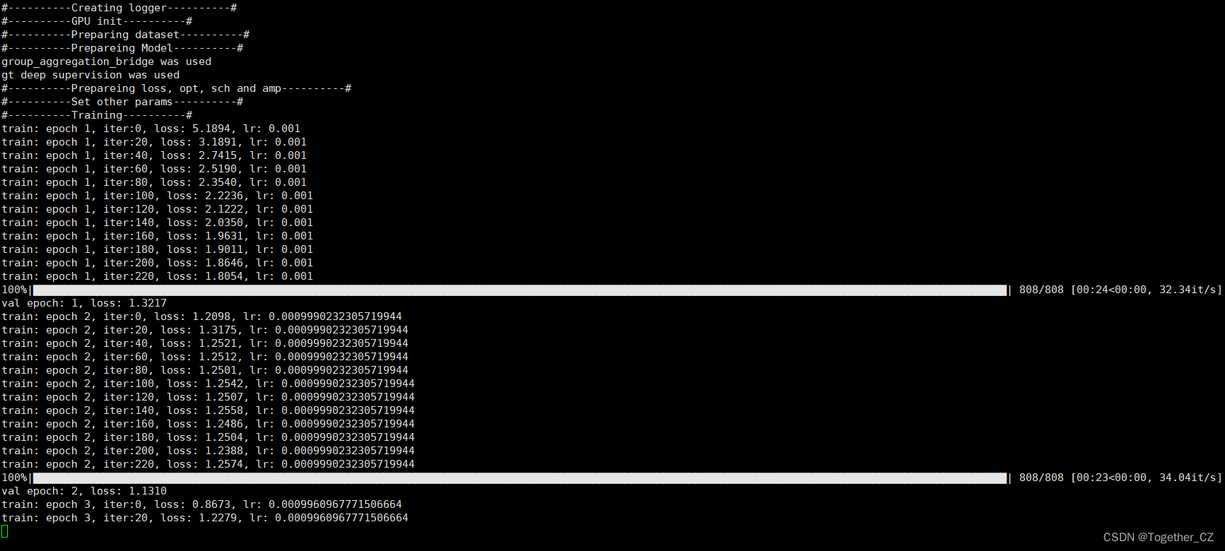
整体的资源占用可以看到还是很低的，如下所示：

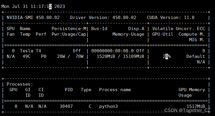
等到模型训练完成后再来看下实际效果，感兴趣的话都可以自己尝试实践一下。后面可以考虑将本文中的超轻量级的模型应用到实际项目开发过程中。

免责声明：本文系网络转载或改编，未找到原创作者，版权归原作者所有。如涉及版权，请联系删