


软件

产品


关于分离变量法求解PDE可以看我前面一篇专栏。
这里给一个用MATLAB求解最简单PDE的代码,设一维杆两端温度保持为0,初始杆温度分为为100度。
%% by LeMonMon 2020/12/27
%% clear command/workspace
clc
clear
%% set paras
global a;
dt = 0.1;
t_max = 20;
dx = 0.01;
x_max = 1;
a = 0.121;
%% init mat
max_i = floor(x_max/dx);
max_j = floor(t_max/dt);
val_u1 = zeros(max_i, max_j);
val_u2 = zeros(max_i, max_j);
%% global var, fourier series don't relay on t
max_terms = 200;
global fourier_series;
fourier_series = zeros(1, max_terms);
% initial condition
phi = @(x) 100;
for n = 1 : max_terms
    ifunc = @(x) phi(x)*sin(n*pi*x);
    fourier_series(n) = 2*solve_int(ifunc, 0, 1, 1000);
end
%% calculate
% only 10 terms
for i = 0 : max_i
    for j = 0 : max_j
        val_u1(i + 1, j + 1) = u1(dx*i, dt*j);
    end
end
% 200 terms
for i = 0 : max_i
    for j = 0 : max_j
        val_u2(i + 1, j + 1) = u2(dx*i, dt*j);
    end
end
E = abs(val_u2 - val_u1);
%% plot
ax = cell(1, 3);
% subplot1: 10 terms
fig = figure(1);
ax{1} = subplot(1,2,1);
x = 0 : dx : x_max;
t = 0 : dt : t_max;
[xx, tt] = meshgrid(x, t);
m1 = mesh(tt', xx', val_u1);
ax{2} = subplot(1,2,2);
m2 = mesh(tt', xx', val_u2);
% error:
fig2 = figure(2);
ax{3} = subplot(1,1,1);
E = abs(val_u2-val_u1);
b = bar3(E, 1);

%% fig/axis set
ax{1}.Title.String = '10 terms';
ax{2}.Title.String = '200 terms';
ax{3}.Title.String = 'difference';
ax{1}.ZLim = [0, 120];
ax{2}.ZLim = [0, 120];
ax{3}.YLim = [0, max_i + 2];
for i = 1 : 3
    ax{i}.XLabel.String = 't';
    ax{i}.YLabel.String = 'x';
    ax{i}.ZLabel.String = 'u';
    ax{i}.FontSize = 16;
    ax{i}.FontName = 'Times New Roman';
    view(ax{i}, [1,-1,.5])
end
%% function
% Use vecterization if possible. It is faster for the reason of CPU
% frameworks.
% function of u, only use the first 10 fourier series
function res = u1(x,t)
    global fourier_series a;
    n = 1:10;
    res = sum(fourier_series(n).*exp(-n.^2*pi^2*a^2*t).*sin(n.*pi*x));
end

% 200 terms
function res = u2(x,t)
    global fourier_series a;
    n = 1:200;
    res = sum(fourier_series(n).*exp(-n.^2*pi^2*a^2*t).*sin(n.*pi*x));
end

% calculate integral using trapezium formula, simply dividing interval to N
% parts
function res = solve_int(f, a, b, N)
    s = (b-a)/N;
    x = a : s : b - s ;
    res = sum(0.5*s.*(f(x)+f(x+s)));
end
整体上通过分离计算Fourier系数和向量化求和,计算速度还是比较可观的。
结果:
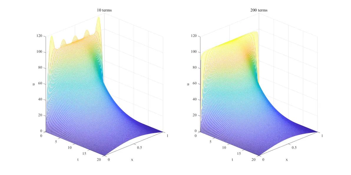
20时间间隔
观察到当时间比较短的时候,可能会导致振荡比较严重,但时间推进,振荡会快速消失。这个情况和Fouier级数计算的项数、数值计算Fourier系数的精度有关。本人能力有限暂不做分析。
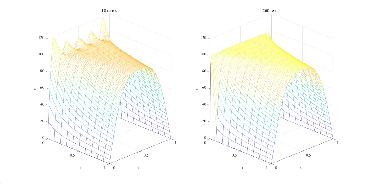
1时间间隔,可以看到最开始几个时间间隔的震荡
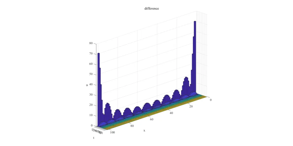
10项和200项的绝对误差,可以看到误差经过前几项快速衰减
武汉格发信息技术有限公司,格发许可优化管理系统可以帮你评估贵公司软件许可的真实需求,再低成本合规性管理软件许可,帮助贵司提高软件投资回报率,为软件采购、使用提供科学决策依据。支持的软件有: CAD,CAE,PDM,PLM,Catia,Ugnx, AutoCAD, Pro/E, Solidworks 等。
 技术文档
技术文档
 推荐好文
推荐好文


 155-2731-8020


