TensorFlow实现线性回归分析

1 前言

在介绍Tensorflow的过程中，笔者并不会想其它书本一样先依次介绍各种API的作用，然后再来搭建一个模型。这种介绍顺序往往会使你在看API介绍时可能不会那么耐烦，因此在今后笔者将会先搭建出模型，再来介绍其中各个API的作用，即带着目的来进行学习。

在接下来的这篇文章中，我们将以波士顿房价预测为例，通过Tensorflow框架来建立一个线性回归模型。当然，模型本身是很简单，并且模型也不是我们所要介绍的，关键是介绍框架的使用。

2 框架介绍

2.0 安装 tensorflow

为了不与其它环境相冲突，建议为Tensorflow1.15重新建立一个新的虚拟环境（详细过程可**参见此处**）。进入虚拟环境后，执行以下命令即可：

pip install tensorflow==1.15.01.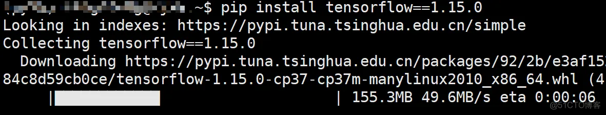

安装完成后在Pycharm中设置相应python解释器（project interpreter）即可，设置过程可参见此处。

2.1 导入相关包

import tensorflow as tffrom tensorflow.keras.datasets.boston_housing import load_datafrom sklearn.preprocessing import StandardScalerimport numpy as np1.2.3.4.

​​tensorflow.keras.datasets​​​中内置了一些比较常用的数据集，并且Tensorflow在各个数据集中均实现了​​load_data​​这个方法来对数据集进行载入。

内置数据集[1]：

Modules​​boston_housing​​ module: Boston housing price regression dataset.​​cifar10​​module: CIFAR10 small images classification dataset.​​cifar100​​module: CIFAR100 small images classification dataset.​​fashion_mnist​​ module: Fashion-MNIST dataset.​​imdb​​IMDB sentiment classification dataset.​​mnist​​module: MNIST handwritten digits dataset.​​reuters​​module: Reuters topic classification dataset.

2.2 载入数据

def load_boston_data():    (x_train, y_train), (x_test, y_test) = load_data(test_split=0.3)    ss = StandardScaler()    x_train = ss.fit_transform(x_train)    x_test = ss.transform(x_test)    return x_train, y_train, x_test, y_test1.2.3.4.5.6.

在对应的数据集下导入​​load_data()​​​方法后，就可以传入参数对数据进行导入。具体参数信息可以查看相应的说明。同时，在这里我们借助了sklearn中的​​StandardScaler()​​来对数据进行标准化。

2.3 定义正向传播

def forward(x, w, b):    return tf.matmul(x, w) + b1.2.

这里的​​tf.matmul()​​​执行的是两个矩阵相乘的操作，同​​np.matmul()​​​一样，接着就是加上偏置。另外，其实Tensorflow中还实现了一个便捷的操作来执行这两步，那就是​​tf.nn.xw_plus_b()​​。

2.4 定义损失

def MSE(y_true, y_pred):    return 0.5*tf.reduce_mean(tf.square(y_true - y_pred))1.2.

这里返回的就是普通的均方误差MSE，并且还除以了2。其中​​tf.square()​​​同​​np.square()​​​一样，计算的是变量的平方；​​tf.reduce_mean()​​​则同​​np.mean()​​​一样用来计算所有元素的平均值，为什么Tensorflow会加上一个前缀​​reduce​​​呢？那是因为​​mean()​​​操作后通常维度都会降低，所以Tensorflow才贴心的在这个操作前加了​​reduce​​​，也有提醒使用者的作用。类似的还有​​tf.reduce_sum()​​​、​​tf.reduce_min()​​​和​​tf.reduce_max()​​等。

2.5 训练模型

def train(x_train, y_train, x_test, y_test):    learning_rate = 0.1    epochs = 300    m, n = x_train.shape    x = tf.placeholder(dtype=tf.float32, shape=[None, n], name='input_x')    y = tf.placeholder(dtype=tf.float32, shape=[None], name='input_y')    w = tf.Variable(tf.truncated_normal(shape=[n, 1],                                        mean=0, stddev=0.1,                                        dtype=tf.float32))    b = tf.Variable(tf.constant(0, dtype=tf.float32, shape=[1]))    y_pred = forward(x, w, b)    loss = MSE(y, y_pred)    train_op = tf.train.GradientDescentOptimizer(learning_rate).minimize(loss)    with tf.Session() as sess:        sess.run(tf.global_variables_initializer())        for epoch in range(epochs):            feed_dict = {x: x_train, y: y_train}            l, _ = sess.run([loss, train_op], feed_dict=feed_dict)            print("[{}/{}]----loss on train:{:.4}".format(epoch, epochs, l))            if epoch % 10 == 0:# 每隔10轮迭代输出一次信息                feed_dict = {x: x_test, y: y_test}# 喂入测试集                l = sess.run(loss, feed_dict=feed_dict)# 计算测试集上的损失                print("[{}/{}]----loss on test:{:.4}-----RMSE: {:.4}".                      format(epoch, epochs, l, np.sqrt(l)))1.2.3.4.5.6.7.8.9.10.11.12.13.14.15.16.17.18.19.20.21.22.23.24.

这部分涉及到Tensorflow的代码最大，我们从上往下依次介绍。

​​tf.placeholder​​

在**上一篇文章**中，我们已经介绍了什么是占位符，但是并没有介绍其用法。在声明一个​​placeholder​​时，我们必须要指定其类型​​dtype​​，形状​​shape​​，以及可选的​​name​​。同时，由于在执行计算图的过程中，每个输入的样本数可能不一样，所以​​shape​​的第一个维度可以设置为​​None​​，例如在训练和测试时​​batch​​的大小可能不一样，如果这种情况下设为定值那么就会报错：

ValueError: Cannot feed value of shape (152, 13) for Tensor ‘input_x:0’, which has shape ‘(354, 13)’

另外需要说明的就是参数​​name​​，它是一个可选参数。在Tensorflow中，几乎所有​​tf.​​打头的类或者方法都有​​name​​这么一个参数（例如​​tf.Variable(),tf.square()​​等），并且都是可选的。因此初学者就会感到奇怪，这个​​name​​到底有什么用，定义变量的时候不是指定了变量名吗？怎么还存在​​name​​这么一个参数？这其实就要从Tensorflow的机制说起，Tensorflow在执行计算图时对于各种变量以及op的识别依赖的就是其对应的名称，而我们定义的变量名只是用于用户角度区分。例如上面​​x=placeholder(...,name='input_x')​​这个占位符，用户通过​​x​​来对其辨识，而Tensorflow内部则是通过​​input_x​​来进行辨识。到目前为止我们并没有发现​​name​​参数的利用价值，但是当实现一些特殊操作时就会体现（后面会有示例）。

​​tf.Variable()​​

​​Variable​​翻译过来就是变量的意思，在Tensorflow中各类网络权重参数都需要通过其来进行定义。同时，​​Variable​​需要传入的第一个参数就是初始值，而​​tf.truncated_normal()​​就是用来对其进行初始化。

​​tf.truncated_normal()​​

截断正太分布，所谓截断就是对不符合条件（大于平均值两个标准差）的值进行舍弃并重新产生。​​mean​​和​​stddev​​分别表示均值和标准差。​​tf.constant()​​则是定义一个常数张量。

​​GradientDescentOptimizer()​​

梯度下降优化器，这里也就是通过梯度下降来对网络的权重进行更新，其至少需要接收一个学习率作为参数。同时，其实例化的​​minimize()​​方法需要传入我们要最小化的损失函数。

​​tf.Session()​​

开启一个会话模式，因为后续我们需要通过​​sess.run()​​来执行计算图。而​​global_variables_initializer()​​则是用于对之前所有定义的​​Variable()​​进行初始化赋值操作（声明的时候并没有完成赋值操作）。

​​feed_dict​​ 对于前面定义的所有的​​placeholder​​，在启动计算图时都需要喂入相应的真实数据。在Tensorflow中，我们将以一个字典的形式把所有占位符需要的东西传进去。注意，字典的key就是占位符的名称，value就是需要传入的值。

​​l,_ = run([loss, train_op])​​

由于我们需要输出查看具体的损失值，所以要将执行​​loss​​的计算；同时，我们需要更新网络权重，所以要执行​​train_op​​这个优化器操作。最后，我们用​​l​​来接收返回的损失值，​​_​​来忽略​​traip_op​​返回的值。

2.6 运行结果

[0/300]----loss on train:294.8[0/300]----loss on test:250.5-----RMSE: 15.83[1/300]----loss on train:247.1[2/300]----loss on train:208.5[3/300]----loss on train:177.3[4/300]----loss on train:151.9[5/300]----loss on train:131.4[6/300]----loss on train:114.8[7/300]----loss on train:101.3[8/300]----loss on train:90.43[9/300]----loss on train:81.59[10/300]----loss on train:74.44[10/300]----loss on test:66.14-----RMSE: 8.1331.2.3.4.5.6.7.8.9.10.11.12.13.

3 总结

在这篇文章中，笔者首先介绍了如何安装Tensorflow1.15；然后依次介绍了实现线性回归中所涉及到的相关Tensorflow知识，包括​​tf.matual()​​​、​​tf.Variable()​​​以及​​GradientDescentOptimizer()​​等等。

免责声明：本文系网络转载或改编，未找到原创作者，版权归原作者所有。如涉及版权，请联系删