利用Python二次开发实现CAE结果的自动化后处理

后处理过程都是基于商业软件进行的，很多数据加工的功能受限于软件的函数接口，因此不够丰富。同时，基于hypergraph或meta的后处理都需要启动软件来完成数据处理，如果进行优化集成则（后台）启动后处理软件也需要一些时间。

这里介绍一些基于Python的CAE结果后处理方法，而不是基于商业软件来完成。包括Nastran结果文件.op2和.pch，LSDYNA结果文件d3plot和binout等自动后处理过程。ABAQUS的开发语言支持Python，因此对于ABAQUS的.odb结果自动后处理就不做过多的介绍。这些自动后处理过程既可用于常规分析自动后处理，也可以用于多学科优化时优化流程的集成，且这些过程不需要商业软件，只需要简单的配置下Python环境即可。

本文介绍基于Python的Nastran结果文件.pch自动后处理，包括IPI、VTF等。

一、IPI自动后处理

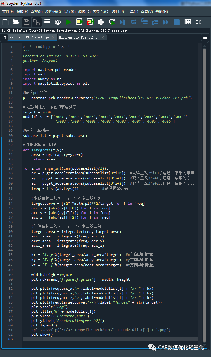
# -*- coding: utf-8 -*-"""Created on Tue Mar  9 12:31:51 2090@author: Ansyent"""import nastran_pch_readerimport mathimport numpy as npimport matplotlib.pyplot as plt#获得pch文件p = nastran_pch_reader.PchParser('F:/07_TempFileCheck/IPI_NTF_VTF/XXX_IPI.pch')#设置动刚度目标值和节点列表target = 7000nodeidlist = ['1001','1002','1003','1004','2001','2002','2003','3001','3002'\              ,'3003','3004','4001','4002','4003','4004','4005','4006']#获得工况列表subcaselist = p.get_subcases()#构造计算面积函数def integrate(x,y):    area = np.trapz(y=y,x=x)    return area
    这里定义了一个计算曲线面积的函数，用于后续动刚度计算。
    

for i in range(int(len(subcaselist)/3)):    ax = p.get_accelerations(subcaselist[3*i+0])  #获得工况3*i+0加速度，结果为字典    ay = p.get_accelerations(subcaselist[3*i+1])  #获得工况3*i+1加速度，结果为字典    az = p.get_accelerations(subcaselist[3*i+2])  #获得工况3*i+2加速度，结果为字典    freq = list(ax.keys())           #获得频率列表

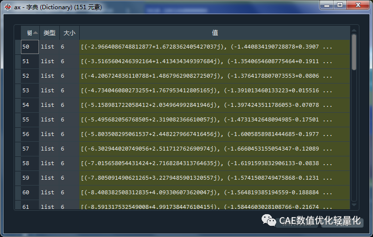
其中ax、ay、az是通过get_accelerations函数得到的一个包含所有分析输出频率个数的字典，字典的键为频率，值为包含六个方向的加速度值，即三个平动三个转动加速度值的列表。并且是通过实部虚部给出的，我们要的是幅值和相位表达，因此后续需要通过abs函数求出对应的幅值。

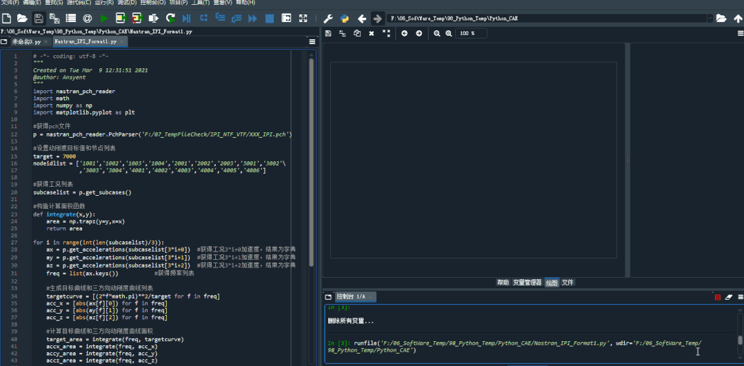
在spyder环境下运行的效果。

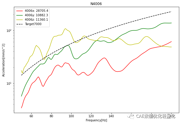
结果图片：

二、VTF自动后处理

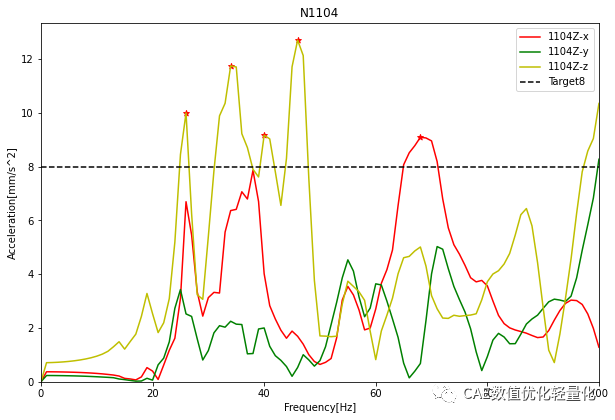
# -*- coding: utf-8 -*-"""Created on Wed Mar 10 13:14:55 2090@author: Ansyent"""import nastran_pch_readerimport scipy.signal as sgnimport matplotlib.pyplot as plt#获得pch文件p = nastran_pch_reader.PchParser('F:/07_TempFileCheck/IPI_NTF_VTF/TB_VTF.PCH')#设置VTF目标值target = 8nodeidlist = ['101','102','201','202','301','302','303','304','501','502'\              ,'503','504','601','602','603','604','1002','1003','1005'\              ,'1006','1007','1101','1102','1103','1104']#获得工况列表subcaselist = p.get_subcases()directionlist = ['X','Y','Z']for j in range(int(len(subcaselist)/3)):    for i , direction in enumerate(directionlist):        acc_motivation = p.get_accelerations(subcaselist[3*j+i])        freq = list(acc_motivation.keys())            targetcurve = [target]*len(freq)        acc_x = [abs(acc_motivation[f][0]) for f in freq]        acc_y = [abs(acc_motivation[f][1]) for f in freq]        acc_z = [abs(acc_motivation[f][2]) for f in freq]                for acc in [acc_x,acc_y,acc_z]:            numpeaks = sgn.find_peaks(acc,distance=3)            xpotion = list(numpeaks[0])            yvalue = [acc[freq.index(i)] for i in xpotion]            for y in yvalue:                if y > target:                    s = plt.scatter(xpotion[yvalue.index(y)], y, marker='*',c='r')
                    这里通过scipy中的find_peaks函数找到不满足目标值的局部极值点，并在图中用红色的*号标记出来。
                    

        width,height=10,6.6        plt.rcParams['figure.figsize'] = width, height            plt.plot(freq,acc_x,'r',label=nodeidlist[j]+direction+"-x")        plt.plot(freq,acc_y,'g',label=nodeidlist[j]+direction+"-y")        plt.plot(freq,acc_z,'y',label=nodeidlist[j]+direction+"-z")        plt.plot(freq,targetcurve,'--k',label="Target" + str(target))        plt.title("N" + nodeidlist[j])        plt.xlabel("Frequency[Hz]")        plt.ylabel("Acceleration[mm/s^2]")        plt.xlim(freq[0],freq[-1])        plt.ylim(bottom=0)        plt.legend()        #plt.savefig('F:/07_TempFileCheck/IPI/' + nodeidlist[i] + '.png')        plt.show()
        

（注：这里只是为了演示，因此把目标值设置为8）。

     以上只是简单介绍了.pch文件的读取和结果自动后处理过程，整个过程只需要几行Python代码即可完成。运行时间也就几秒钟。而不需要在商业软件中来进行。如果是进行优化集成，则不要输出结果图片等信息，只需要输出结果响应即可，会大大提高效率。同时，如果需要自动生成报告和结果统计等，只需要在次基础上添加简单的几行命令即可，十分方便简洁。

后续介绍ls-dyna结果d3plot和binout自动后处理方法。

免责声明：本文系网络转载或改编，未找到原创作者，版权归原作者所有。如涉及版权，请联系删